Solar availability at geostationary orbit

Let us consider a solar satellite orbiting in geostationary orbit, which is located at a distance of around 35,000 km. Because a geostationary satellite always orbits above the equator (which we call its orbital plane), and the Earth is tilted, the Earth’s shadow does not actually block sunlight. We have a diagram below to show this:

Because the Earth’s rotational axis is tilted by an angle of $\varphi \approx 23.44°$, the geostationary orbit lies above a straight-line plane drawn through an Earth (known as the plane of reference). We can in fact calculate its height above the reference plane as follows. Using trigonometry, it is possible to show that the satellite’s angle of elevation ${\theta }_{\text{sat}}$ above the reference plane satisfies ${\theta }_{\text{sat}}={\varphi }_e$. We may derive this as follows: since the Earth’s axis is perpendicular to the satellite’s orbital plane, while a vertical line through the Earth is perpendicular to the plane of reference. Thus:

$$\begin{array}{rl}{\varphi }_e^{\prime }& =90°-{\varphi }_e\\ {\theta }_{\text{sat}}& =90°-{\varphi }_e^{\prime }\\ & =90°-(90°-{\varphi }_e)\\ & ={\varphi }_e\end{array}$$

Therefore, by simple trigonometry, the height of the satellite above the reference plane is given by:

$$h=D\sin ({\theta }_{\text{sat}})=D\sin ({\varphi }_e)\approx \text{16,772.4 km}$$

Where $D\approx 42,164$ $\mathrm{km}$ is the satellite’s orbital distance relative to the center of the Earth (we may derive this from the equations of uniform circular motion). Meanwhile, we will derive the height of the Earth’s shadow (using our idealized model of a perfect solar beam; in reality, diffraction modifies this, but we’ll use this approximation for now, and calculate the corrections later). The angle ${\varphi }_s$ made by the Earth’s shadow with respect to the plane of reference would be given by:

$${\varphi }_s={\tan }^{-1}\left(\frac{R_e}{s}\right)$$

Where $R_e\approx 6,357\mathrm{km}$ is the Earth’s radius at the North Pole, and $s\approx 1.4\times 10^6\mathrm{km}$ is the length of Earth’s umbra. Using our diagram, the height of the Earth’s shadow above the plane of reference directly above the plane of reference becomes $b=R_e-a$, where:

$$\begin{array}{rl}\tan ({\varphi }_s)& =\frac{a}{D\cos ({\theta }_{\text{sat}})}\\ & \Rightarrow a=D\cos ({\varphi }_e)\tan ({\varphi }_s)\\ & =D\cos ({\varphi }_e)\left(\frac{R_e}{s}\right)\end{array}$$

From this, we find that $b\approx 6181.1\mathrm{km}\ll h$; in fact, the satellite orbits more than 10,000 km above the Earth’s shadow. Therefore, at least for much of the year, the satellite experiences 24-hour sunlight. The reason why we say much of the year instead of all of the year is that in our calculations, we didn’t include the orbital inclination of the Earth. As the Earth itself doesn’t perfectly rotate in the ecliptic plane (the reference plane of the Solar System), but rather, orbits at ${\Omega }_i=7.155°$ above it, the overall angle will change. The effective tilt of the Earth, therefore, is not ${\varphi }_e$, but rather ${\varphi }_e+{\varphi }_i(t)$, where ${\varphi }_i(t)$ is the additional angle caused by the Earth’s angled orbital plane (which in general is a function of time); this effect is shown in the below diagram:

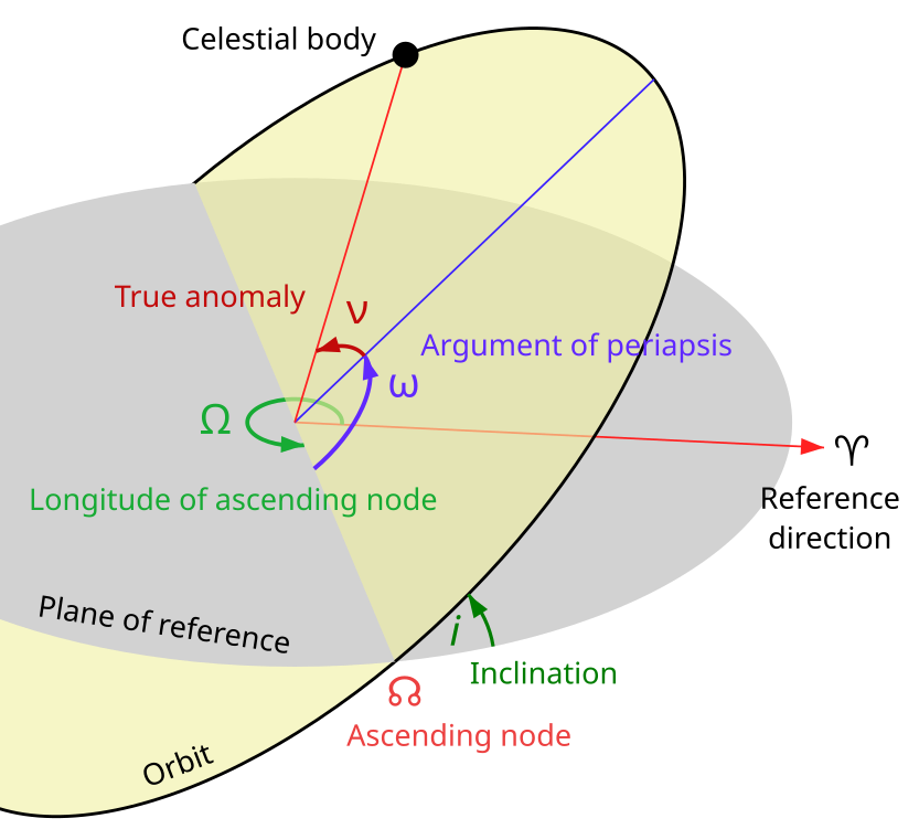
Source: Wikipedia

The additional angle can be found using trigonometry from the true anomaly $\nu (t)$ and the orbital radius $r$, which is a function of time. Using trigonometry, the height of the Earth above the ecliptic is given by:

$$h^{\prime }=(r\sin \nu )\sin {\Omega }_i$$

This nonzero height leads to the shadow height $b$ gaining an additional height $\Delta y=(r\sin \nu )\sin {\Omega }_i$. The result is that in a 1-month period around those two days of the year, near the solar equinoxes (when the Earth passes through the ecliptic), the satellite will be in the dark for a short period of time (about an hour at maximum, usually less). However, for the other ~10 months of the year, it will not be affected. This issue can readily be solved by having a constellation of satellites

Also, note that as stated earlier, we did not account for diffraction. If we account for the effects of diffraction, the calculations become much more involved as we then need to solve the full Helmholtz equation (no approximations!) with the boundary condition $u(x,y,0)=0$ for all $x^2+y^2=R_e$, which is so complicated that we might as well solve it numerically. However, the main result is that the scattering of the Sun’s light due to diffraction leads to a semi-transparent shadow that spreads wider than the main shadow. There will still be 24-hour sunlight here; it will just be a percentage weaker than the standard solar irradiance (the power output by the Sun received at Earth) of $1.362$ $kW/{\mathrm{m}}^2$.

Atmospheric optical path length

Another factor we need to consider is that we want to design the power satellites to beam power to multiple locations instead of just one. This means that we want to have satellite transmitters that can be aimed. Since the satellites sit stationary at geostationary orbit, this capability makes the satellites far more efficient: one satellite with multiple beams can serve multiple cities or even a small country.

However, an important factor in multi-location beaming is the increased distance the beam must travel through the atmosphere. We will now show a derivation of this. First, a diagram of the system is shown below:

We aim to solve for $d$, the optical path length (distance travelled by the beam) through the atmosphere. More precisely, we are interested in the path length through the troposphere, the lowest and densest layer of the atmosphere, where essentially all of the weather we experience occurs (including storms, clouds, rain, hurricanes, etc.). The upper levels of the atmosphere are unimportant to us, since there is effectively no weather there and thus there is little to attenuate our power beams.

Note: There is one exception: the ionosphere, located in Earth’s upper atmosphere, has the ability to reflect certain types of radio waves and microwaves. However, this is not as much of an issue for us, since it primarily reflects HF signals (ranging from $\text{3 MHz}-\text{30 MHz}$) instead of the UHF signals ($\text{1 GHz}$ range) that we are operating at. Indeed, NASA’s Deep Space Network uses S-band microwaves (that is, $2-\text{4 GHz}$ signals) to communicate to spacecraft, which is quite close to our desired frequencies

In our following derivation, the $y$ axis will be the vertical axis; for representational simplicity we will mostly be using $y\le 0$ (that is, the lower quadrants of the Cartesian plane). We will use the following symbols (refer to the previous diagram for a visual):

Symbol	Definition
$d$	Optical path length through atmosphere
$D$	Height of geostationary orbit above the Earth’s surface (defined to be 35,786 km)
$R_{earth}$	Mean radius of the Earth (defined to be 6,371 km)
$h$	Thickness of the troposphere (around 13 km on average). In the special case in which the satellite’s power beam is pointing straight down, $d=h$.
$h_{atmosphere}$	Height of the top of the troposphere, relative to the Earth’s center. By definition, $h_{atmosphere}=R_{earth}+h$
$h_{orbit}$	Orbital height of the satellite, relative to the Earth’s center. By definition, $h_{orbit}=R_{earth}+D$.
$\varphi$	Angle measured from the $-x$ axis to a point on the circle representing the Earth. By convention, we assume that $\varphi \ge 0$.
$\theta$	Angle at which a ray (power beam) from the satellite is tilted, relative to the $y$ axis. We will later show that $\Vert \theta \Vert \le \varphi$.
$H(x)$	Equation of ray travelling at angle $\theta$ from the $y$ axis
$a$	$x$-coordinate of the point where the ray $H(x)$ intersects with a circle of radius $R_{earth}$. Physically, this represents the location the power beam reaches the ground.
$b$	$x$-coordinate of the point where the ray $H(x)$ intersects with a circle of radius $h_{atmosphere}$. Physically, this represents the location the power beam reaches the top of the troposphere.
$T(x)$	Equation of tangent line to the circle representing Earth. Physically, this represents the “grazing beam” i.e. the power beam to the furthest point on Earth the beam can reach, since the curvature of the Earth prevents a straight beam from reaching anywhere further.
To begin, from the aforementioned diagram and some trigonometry, it is not hard to see that $H(x)$ must take the form:

$$H(x)=-h_{orbit}-\cot \left(\theta \right)x$$

The optical path length $d$ is equal to the distance between the point where the ray (power beam) reaches the troposphere and the point where it reaches the ground. Thus, by Pythagoras’s theorem, we have:

$$d=\sqrt{(b-a{)}^2+(H(b)-H(a){)}^2}$$

To find $a$ and $b$, we recall that the equation of a circle centered at the origin can be written as $x^2+y^2=R^2$. The lower half of a circle can thus be written as $y=-\sqrt{R^2-x^2}$. We can represent the Earth as a perfect circle of radius $R_{earth}$, and the top of the troposphere as a smooth layer on top of the Earth, so it can be modelled as a perfect circle of radius $R=h_{atmosphere}$. Then, $a$ is thus the intersection point of the ray $H(x)$ with the smaller circle (of radius $R=R_{earth}$), so we have:

$$H(x)=-\sqrt{R_{earth}^2-a^2}$$

Meanwhile, $b$ is thus the intersection point of the ray $H(x)$ with the larger circle (of radius $R=h_{atmosphere}$), so we have:

$$H(x)=-\sqrt{h_{atmosphere}^2-b^2}$$

Thus we have the following two equations to solve:

$$\begin{array}{c}H(x)+\sqrt{R_{earth}^2-a^2}=0\\ H(x)+\sqrt{h_{atmosphere}^2-b^2}=0\end{array}$$

The solutions are quite complicated (see the notebook orbital-trajectory-planning.ipynb in the notebooks/ folder of the parent directory for the calculations), but they are given by:

$$\begin{array}{rl}a& =\left(-h_{orbit}\cdot \frac{1}{\tan \left(\theta \right)}+{\left(\frac{R_{earth}^2}{{\sin }^2\left(\theta \right)}-h_{orbit}^2\right)}^{1/2}\right){\sin }^2\left(\theta \right)\\ b& =\left(-h_{orbit}\cdot \frac{1}{\tan \left(\theta \right)}+{\left(\frac{h_{atmosphere}^2}{{\sin }^2\left(\theta \right)}-h_{orbit}^2\right)}^{1/2}\right){\sin }^2\left(\theta \right)\end{array}$$

Now using our previously-derived expression for $d$, by substituting in the values of $a$ and $b$ we have (after tedious calculation):

$$d={\left[z^2-2h_{orbit}^2{\sin }^2\left(\theta \right)-2{\sin }^2\left(\theta \right)\sqrt{\left(\frac{R_{earth}^2}{{\sin }^2\left(\theta \right)}-h_{orbit}^2\right)\left(\frac{h_{atmosphere}^2}{{\sin }^2\left(\theta \right)}-h_{orbit}^2\right)}\right]}^{1/2}$$

Where we have defined $z^2\equiv R_{earth}^2+h_{atmosphere}^2$. This complicated expression can be approximated (for small values of $\theta$) with:

$$d\approx {\left[h^2-2h_{orbit}^2{\theta }^2-2\alpha \left(\frac{h_{orbit}^2}{2R_{earth}^2}+\frac{h_{orbit}^2}{2h_{atmosphere}^2}\right){\theta }^2\right]}^{1/2}$$

Where we have defined ${\rho }^2$ as:

$$h^2=z^2-2\alpha =R_{earth}^2+h_{atmosphere}^2-2\alpha$$

Taking the limit $\theta \to 0$, we obtain the expected result:

$$d=h$$

Now, we are interested in how much greater $d$ is compared to $h$. That is, what is the value of $d/h$? If we just plug in numbers, we find that $d/h\approx 2$ at a beam angle of around $\theta =35^{\circ }$ with toy values of $R_{earth},h,h_{orbit}$ of order unity (meaning numbers reasonably close to one). This means that the optical path length through the atmosphere at such an angle is double that of the path length had the beam been pointed directly down at Earth (that is, when $\theta =0$). With realistic values of Earth’s radius and the thickness of the actual troposphere, we find that $d/h$ is (surprisingly) still quite close to 2 for most angles within reach of the satellite!

To find a theoretical upper bound on the maximum physically-possible value of $d/h$, we will need to do some more complicated calculations. The furthest possible point on Earth the beam can reach (without unrealistically tunneling through the interior of the Earth) is located at the point of tangency of a circle of radius $R_{earth}$, the point where a tangent line grazes the edge of the circle. We’ll call this point of tangency $B=(B_x,B_y)$. The equation of the tangent line is then given by:

$$T(x)=B_y+B_x\frac{B_x}{B_y}-\frac{B_x}{B_y}x$$

Now, we can parametrize $B$ in another way by noting that it can also be written as $B=(-R_{earth}\cos \varphi ,-R_{earth}\sin \varphi )$ (the negative sign is due to the fact that we are working with the regions under the $x$ axis). By substituting, we can then write $T$ in terms of $R_{earth}$ and $\varphi$. Together with the condition that the tangent line must pass through the location of the satellite (which is located at $x=0$, $y=-h_{orbit}$), meaning that $T(0)=-h_{orbit}$, we can thus solve for $\varphi$ explicitly. Again, the calculation is in the aforementioned notebook, but the result is:

$$\varphi =2\arctan \left(\frac{h_{orbit}-\sqrt{-R_{earth}^2+h_{orbit}^2}}{R_{earth}}\right)$$

Importantly, note that $\varphi$ is the maximum angle that $\theta$ can be before the satellite beam loses contact with the Earth’s surface (due to the curvature of the Earth), and therefore it sets a natural limit on the furthest point on Earth that the satellite can beam to. Thus, we conclude that $|\theta |\le \varphi$. By substituting real values of $h_{orbit}$ and $R_{earth}$ (as we specified in our table at the beginning of this section), we have $\varphi \approx 8.69^{\circ }$, and thus $|\theta |\le 8.69^{\circ }$.

Note: We can derive this by showing that in the limit $\theta \to \varphi$, we have $H(x)\to T(x)$ and thus form a set of similar triangles, for which $\theta$ and $\varphi$ are therefore congruent angles. See this Desmos visualization to see this more easily (try increasing $\theta$ until it is close to equal to $\varphi$).

By now substituting our result into $B_x=-R_{earth}\cos \varphi$, we therefore find that the $x$-coordinate of the furthest point on the Earth’s surface that the beam can reach (equivalently, the $x$ coordinate of the point of tangency) is given by:

$$x_{\text{furthest}}=-\frac{R_{earth}\left(\frac{R_{earth}^2}{h_{orbit}}-h_{orbit}+\sqrt{-R_{earth}^2+h_{orbit}^2}\right)}{h_{orbit}-\sqrt{h_{orbit}^2-R_{earth}^2}}$$

We find that $|x_{\text{furthest}}|\approx \text{6297 km}$, which is (quite impressively!) close to 99% of Earth’s radius. We can then calculate the effective land area this allows the beam to reach. The surface area of a hemisphere is given by $A=2\pi R^2$, where $R$ is its radius. Thus, by setting $R=|x_{\text{furthest}}|$, we obtain an land area of $A=2.492\times 10^8{\text{ km}}^2$. Compared with the total surface area of a hemisphere of the Earth, which is given by $A_{hemi}=2.55\times 10^8{\text{ km}}^2$, we find that $A/A_{hemi}\approx 97.7$.

Note: Here, we use the word “land” loosely, since we mean “land” as in “a part of the Earth’s surface” as opposed to “terrestrial and habitable region”.

This means that one satellite¹ would be in theory sufficient to beam power to close to 98% of a hemisphere, or equivalently, two satellites could beam power to nearly the entire Earth’s surface! However, $d/h$ grows without bound as $\theta$ approaches very close to $\varphi$, meaning that realistically we would like to keep $\theta \le 7.7^{\circ }$, where $d/h\approx 2.15$. Then, we have $|x_{furthest}|=\left|\frac{a\tan \theta }{R_{earth}}\right|\approx \text{5202 km}$. Using the same hemisphere area calculation method as before, a single satellite could then cover a land area of $A=1.7\times 10^8{\text{ km}}^2$, or around 67% of a hemisphere. In that case, we would need three power satellites to make sure we can beam power to anywhere on Earth, although the increase of just one more satellite (compared to the ideal case) is not bad at all!

Note: Of course, remember this entire analysis is under idealized conditions where we simplify the geometry of the Earth and ignore any diffractive effects or beam imperfections. However, it should serve as a good baseline value.

---

Additional thought: Note that Strauss’s textbook Partial Differential Equations, ed. 2 has a section (pg. 367) called “Scattering of plane wave by a sphere”, that might be a helpful read. The important quantity is the falloff, that is, how quickly does the intensity of the sunlight decrease as it diffracts around the planet? After all, our analysis assumed that the beam can be well-modelled by a ray (which is a valid assumption for a tightly-collimated laser/maser beam), but the Sun’s radiation is much more complicated since it emits (effectively) spherical waves which are plane waves by the time they reach Earth, due to the Sun’s immense size and the astronomical distance between Earth and the Sun.

Answer: More information available at https://en.wikipedia.org/wiki/Solar_irradiance

Footnotes

1. More realistically, it wouldn’t be one satellite, but one satellite cluster: a group of tightly-packed power satellites orbiting together. ↩