Solving for the fields in a hollow waveguide

For the output coupler of our maser (see Satellite maser engineering), we will need some form of output coupler that guides the microwaves out of the maser so we have a nice and focused beam. This will probably take the form of a hollow RF waveguide, with the left end attached to the maser, and the right end being an open end to allow the microwave beam to propagate away and out of the maser.

The general materials for a microwave waveguide can be essentially any type of metal, since metals in general are all highly-reflective of microwaves. However, there are other important design considerations. For instance, if we have a waveguide, is it more advantageous for it to have a constant radius (that is, take the shape of a cylindrical tube), or for it to be either widen or shrink along its length? A diagram of these three possible configurations is shown below:

This is actually a surprisingly difficult question to answer rigorously. However, it turns out that we can actually work out the solution analytically, with patience and a huge load of math. Let’s dive in!

Mathematical setup

To start, we will be solving the Helmholtz equation, which governs the spatial propagation of electromagnetic waves (it is the time-independent electromagnetic wave equation). The Helmholtz equation for the electric field can be written in its most general form as:

$$({\nabla }^2+k^2)\mathbf{E}=0$$

Where $k=2\pi /\lambda$ is the wavenumber of the wave, and is the magnitude of the wavevector $\mathbf{k}$, which points in the direction of travel of the wave. We use the coordinate system shown in the diagrams at the top of the page, and since our waveguides are radially-symmetric, we’ll use cylindrical coordinates $(r,\varphi ,z)$. Additionally, we’ll be solving the scalar version of the Helmholtz equation:

$$({\nabla }^2+k^2)E_{\perp }=0$$

Where $E_{\perp }=E_{\perp }(r,\theta ,\varphi )$ is the transverse component of the electric field (perpendicular to the $z$ axis), since we assume that the electric field is purely transverse. For this reason, we’ll use the slopping notation of just calling $E_{\perp }$ the “electric field” and writing it as $E$, since we don’t care about the longitudinal component (which is zero). Thus, with this convention, the Helmholtz equation can be written as:

$$({\nabla }^2+k^2)E=0$$

If we expand the Laplacian in cylindrical coordinates, we have:

$$\frac{1}{r}\frac{\partial E}{\partial r}+\frac{{\partial }^{2}E}{\partial r^2}+\frac{1}{r^2}\frac{{\partial }^{2}E}{\partial {\varphi }^2}+\frac{{\partial }^{2}E}{\partial z^2}+k^{2}E=0$$

Now let’s write down the boundary conditions for the problem. We assume cylindrical symmetry, so we know that $E(r,\varphi ,z)=E(r,\varphi +2\pi ,z)$, which is a periodic boundary condition. Additionally, as the waveguide is made of metal, we know the electric field must vanish at the edge of the waveguide. The edge of the waveguide can be described by a function $R(z)$, which is given by:

$$R(z)=a+z\tan \theta ,0\le z\le L$$

Where $a$ is the radius of the waveguide at the end attached to the maser, $L$ is the horizontal length of the waveguide, and $\theta$ (as shown in the diagram at the top) is the angle the edge of the waveguide makes with the horizontal axis. Thus, our second boundary condition is $E(R(z),\varphi ,z)=0$. Putting these two boundary conditions together, we get:

$$\begin{array}{c}E(r,\varphi ,z)=E(r,\varphi +2\pi ,z)\\ E(R,\varphi ,z)=0,R=R(z)\end{array}$$

Separation of variables

To solve the Helmholtz equation, we will use the technique of separation of variables. We assume that the solution $E(r,\varphi ,z)$ takes the form:

$$E(r,\varphi ,z)=\psi (r,z)\Phi (\varphi )$$

This means that the partial derivatives of the electric field are given by:

$$\begin{array}{rl}\frac{\partial E}{\partial r}& =\frac{\partial \psi }{\partial r}\Phi \\ \frac{{\partial }^{2}E}{\partial r^2}& =\frac{{\partial }^2\psi }{\partial r^2}\Phi \\ \frac{{\partial }^{2}E}{\partial {\varphi }^2}& ={\Phi }^{\prime \prime }\psi \\ \frac{{\partial }^{2}E}{\partial z^2}& =\frac{\partial {\psi }^2}{\partial z^2}\Phi \end{array}$$

After substituting our partial derivatives into the Helmholtz equation and multiplying both sides of the PDE by $\frac{1}{\Phi \psi }$, we have:

$$\begin{array}{c}\frac{1}{r}\Phi \frac{\partial \psi }{\partial r}+\frac{{\partial }^2\psi }{\partial r^2}\Phi +\frac{1}{r^2}{\Phi }^{\prime \prime }\psi +\frac{{\partial }^2\psi }{\partial z^2}\Phi =-k^2\Phi \psi \\ \frac{1}{\Phi \psi }\left[\frac{1}{r}\Phi \frac{\partial \psi }{\partial r}+\frac{{\partial }^2\psi }{\partial r^2}\Phi +\frac{1}{r^2}{\Phi }^{\prime \prime }\psi +\frac{{\partial }^2\psi }{\partial z^2}\Phi \right]=-k^2\frac{1}{\Phi \psi }\Phi \psi \\ \frac{1}{r\psi }\frac{\partial \psi }{\partial r}+\frac{1}{\psi }\frac{{\partial }^2\psi }{\partial r^2}+\frac{1}{r^2}\frac{{\Phi }^{\prime \prime }}{\Phi }+\frac{1}{\psi }\frac{{\partial }^2\psi }{\partial z^2}=-k^2\\ \frac{1}{r\psi }\frac{\partial \psi }{\partial r}+\frac{1}{\psi }\frac{{\partial }^2\psi }{\partial r^2}+\frac{1}{\psi }\frac{{\partial }^2\psi }{\partial z^2}=-\left(\frac{1}{r^2}\frac{{\Phi }^{\prime \prime }}{\Phi }+k^2\right)=\alpha m^2\end{array}$$

Where $m^2$ is some constant, and we use $\alpha m^2$ where $\alpha =\pm 1$ because we will pick the physically-relevant sign later. This now gives us two differential equations:

$$\begin{array}{c}\frac{1}{r^2}\frac{{\Phi }^{\prime \prime }}{\Phi }+k^2=-\alpha m^2\\ \frac{1}{r\psi }\frac{\partial \psi }{\partial r}+\frac{1}{\psi }\frac{{\partial }^2\psi }{\partial r^2}+\frac{1}{\psi }\frac{{\partial }^2\psi }{\partial z^2}=\alpha m^2\end{array}$$

We can write them in a more readable form as:

$$\begin{array}{c}\frac{d^2\Phi }{d{\varphi }^2}=-r^2{n}^2\Phi ,n^2=\alpha m^2+k^2\\ {\nabla }^2\psi +\frac{1}{r}\frac{\partial \psi }{\partial r}=\alpha m^2\psi \end{array}$$

Where ${\nabla }^2\psi ={\psi }_{rr}+{\psi }_{zz}$ is the 2D Laplacian. Notice that we still have a PDE for $\psi (r,z)$ left - so we’ll need to repeat the separation of variables procedure again.

Note: Yes, technically this is not the “correct” way to do separation of variables since we haven’t fully separated the variables, so the differential equation for $\Phi$ depends on $\varphi$ and $r$. However, it doesn’t seem to matter for the physical result (probably because of the periodic boundary condition that allows us to regard $r=\text{const.}$ for all intents and purposes when solving for $\Phi (\varphi )$, the angular function). More discussion on this would be helpful.

Separation of variables for $\psi (r,z)$

For the PDE, we again perform the standard separation of variables by assuming $\psi (r,z)$ to take the form $\psi (r,z)=W(r)Z(z)$. Then, ${\nabla }^2\psi =W^{\prime \prime }Z+Z^{\prime \prime }W$, and $\frac{\partial \psi }{\partial r}=W^{\prime }Z$. This gives us:

$$W^{\prime \prime }Z+Z^{\prime \prime }W+\frac{1}{r}{W}^{\prime }Z=\alpha m^{2}WZ$$ $$\frac{1}{WZ}\left[W^{\prime \prime }Z+Z^{\prime \prime }W+\frac{1}{r}{W}^{\prime }Z\right]=\frac{1}{WZ}\alpha m^{2}WZ$$ $$\frac{W^{\prime \prime }}{W}+\frac{Z^{\prime \prime }}{Z}+\frac{1}{r}\frac{W^{\prime }}{W}=\alpha m^2$$ $$\frac{W^{\prime \prime }}{W}+\frac{1}{r}\frac{W^{\prime }}{W}=\alpha m^2-\frac{Z^{\prime \prime }}{Z}=\beta {\ell }^2$$

Where ${\ell }^2$ is some other constant, and again $\beta =\pm 1$, where we’ll pick the sign later. This gives us another two ODEs:

$$\begin{array}{c}\frac{W^{\prime \prime }}{W}+\frac{1}{r}\frac{W^{\prime }}{W}=\beta {\ell }^2\\ \frac{Z^{\prime \prime }}{Z}-\alpha m^2=-\beta {\ell }^2\end{array}$$

We can write these in a more readable form as:

$$\begin{array}{c}\frac{d^{2}W}{d{r}^2}+\frac{1}{r}\frac{dW}{dr}=\beta {\ell }^{2}W(r)\\ \frac{d^{2}Z}{d{z}^2}=-(\beta {\ell }^2-\alpha m^2)Z\end{array}$$

Solving for $W(r)$

Note that the first of our two differential equations can be slightly rearranged by multiplying by $r^2$ on all sides and setting the right-hand side to zero. This yields:

$$r^2\frac{d^{2}W}{d{r}^2}+r\frac{dW}{dr}-r^2\beta {\ell }^{2}W(r)=0$$

A quick search shows that this is a zeroeth-order Bessel differential equation, whose solution can be written in terms of a Bessel function of the first kind, $J_0(r)$:

$$W(r)=C_1{J}_0(r\sqrt{-\beta {\ell }^2})$$

We now know that we must choose $\beta =-1$ for our solution to be physically-valid (otherwise the square root is imaginary). Thus, we have:

$$W(r)=C_1{J}_0(\ell r)$$

Solving for $Z(z)$

Let’s now solve the next differential equation for $Z(z)$, which, as a reminder, is given by:

$$\frac{d^{2}Z}{d{z}^2}=-(\beta {\ell }^2-\alpha m^2)Z$$

Again, since we found previously that $\beta =-1$, this reduces to:

$$\frac{d^{2}Z}{d{z}^2}=({\ell }^2+\alpha m^2)Z$$

Now, if we choose $\alpha =+1$, then this differential equation would reduce to $Z^{\prime \prime }=({\ell }^2+m^2)Z$, whose solution is in terms of real exponentials in the form $e^z$ or $e^{-z}$. This would lead to a solution that either blows up or decays to zero quickly, which we know cannot happen from the physics since those don’t lead to propagating electromagnetic waves (which must be sinusoidal). Instead, we must choose $\alpha =-1$, so that this differential equation reduces to:

$$\frac{d^{2}Z}{d{z}^2}=({\ell }^2-m^2)Z=-(m^2-{\ell }^2)Z$$

That minus sign makes all the difference, because it means that the solutions are given by complex exponentials that do describe propagating waves (we take the real part of the complex exponential once when we’re done with the calculation, since only the real part is physically-relevant). Since this is just the differential equation of a harmonic oscillator, the solution is given by:

$$Z(z)=C_2{e}^{-i\left(\sqrt{m^2-{\ell }^2}\right)z}$$

Note: The choice of $-i$ or $+i$ is arbitrary since it has no effect on the real part, it’s just a matter of convention.

Solving for $\Phi (\varphi )$

We now solve the last differential equation for $\Phi (\varphi )$. As a reminder, it is given by:

$$\frac{d^2\Phi }{d{\varphi }^2}=-r^2(\alpha m^2+k^2)\Phi$$

With $\alpha =-1$ (as we found previously), this reduces to:

$$\frac{d^2\Phi }{d{\varphi }^2}=-r^2(k^2-m^2)\Phi$$

Interestingly, we don’t really even need to solve this differential equation (although it’s not hard to, since it’s just a harmonic oscillator), since we know that given our periodic boundary condition $\Phi (\varphi )=\Phi (\varphi +2\pi )$, the solution must be a periodic function (a sine or cosine). Let us assume a solution in the form $\Phi (\varphi )=\sin (\xi \varphi )$, where $\xi$ is some constant. Its second derivative is given by ${\Phi }^{\prime \prime }(\varphi )=-{\xi }^2\sin (\xi \varphi )$. With some pattern-matching with our differential equation ${\Phi }^{\prime \prime }=-r^2(k^2-m^2)\varphi$, this gives us:

$${\xi }^2=r^2(k^2-m^2)\Rightarrow \xi =r\sqrt{k^2-m^2}$$

So indeed this is a valid solution. Substituting in our boundary condition, we have:

$$\Phi (\varphi +2\pi )=\sin (\xi (\varphi +2\pi ))=\sin (\xi \varphi )$$

Expanding with the trigonometric identity $\sin (A+B)=\sin A\cos B+\cos A\sin B$, this expands to:

$$\sin (\xi \varphi )\cos (2\pi \xi )+\cos (\xi \varphi )\sin (2\pi \xi )=\sin (\xi \varphi )$$

To make this equation valid, we must have $\cos (2\pi \xi )=1$ and $\sin (2\pi \xi )=0$. Luckily, these two conditions are equivalent - sine is always zero when cosine is one, and vice-versa - so as long as we fulfill one condition, we fulfill both. Sine is zero at all intervals $j\pi$ where $j$ is an integer, so the condition is satisfied with $2\pi \xi =j\pi$, or $\xi =j/2$. Thus, we have:

$$\Phi (\varphi )=\sin (\xi \varphi )=\sin (j\varphi /2)$$

Since $\xi =j/2\iff j=2\xi =2r\sqrt{k^2-m^2}$ this solution can equivalently be written as:

$$\Phi (\varphi )=C_3\sin (r\left(\sqrt{k^2-m^2}\right)\varphi )$$

Where $C_3$ is some arbitrary separation constant. We’ve now solved all of our differential equations!

Combined solution

Combining our separate solutions for $W(r),Z(z)$, and $\Phi (\varphi )$, we have:

$$\begin{array}{rl}E(r,\varphi ,z)& =\psi (r,z)\Phi (\varphi )\\ & =W(r)Z(z)\Phi (\varphi )\\ & =C_{m\ell }{J}_0(\ell r)\sin (r\left(\sqrt{k^2-m^2}\right)\varphi )e^{-i\left(\sqrt{m^2-{\ell }^2}\right)z}\end{array}$$

Where we have absorbed the constants $C_1,C_2,C_3$ into a generic constant $C_{m\ell }$. This gives us the set of solutions:

$$E_{m,\ell }(r,\varphi ,z)=C_{m\ell }{J}_0(\ell r)\sin (r\left(\sqrt{k^2-m^2}\right)\varphi )e^{-i\left(\sqrt{m^2-{\ell }^2}\right)z}$$

Now, remember that our other boundary condition was given by:

$$E(R,\varphi ,z)=0,R(z)=a+z\tan \theta ,a,z=\text{const}$$

Where $a,\theta$ are constants. If we substitute this in, we have:

$$E_{m,\ell }(R(z),\varphi ,z)=C_{m\ell }{J}_0(\ell (a+z\tan \theta ))\sin \left(\left(a+z\tan \theta )\sqrt{k^2-m^2}\right)\varphi \right)e^{-i\left(\sqrt{m^2-{\ell }^2}\right)z}=0$$

This is satisfied in general only if:

$$\sin \left(\left(a+z\tan \theta )\sqrt{k^2-m^2}\right)\varphi \right)=0$$

Which requires that:

$$(a+z\tan \theta )\left(\sqrt{k^2-m^2}\right)\varphi =n\pi ,n=0,1,2,3,\dots$$

This is an implicit equation that constrains $z$ and $\varphi$, which can be rearranged into the form:

$$\varphi =\frac{n\pi }{(a+z\tan \theta )\sqrt{k^2-m^2}}$$

Thus, our radial function becomes:

$$E_{n,\ell ,m}(r,\varphi ,z)=C_{m\ell }{J}_0(\ell r)\sin \left(\frac{n\pi r}{a+z\tan \theta }\varphi \right)e^{-i\left(\sqrt{m^2-{\ell }^2}\right)z}$$

If we consider purely the radial component (let’s call it $Q(r)$, we’re ignoring $z$) at a slice $\varphi =1$, we have:

$$Q(r)=J_0(\ell r)\sin \left(\frac{n\pi r}{a+z\tan \theta }\right)$$

A plot of this function (excluding the Bessel function, the function exhibits the same qualitative characteristics without it) can be found on this interactive Desmos visualization. In addition, a plot with the parameters $a=0.5,n=1,\ell =1,\theta =pi/3$ is shown below:

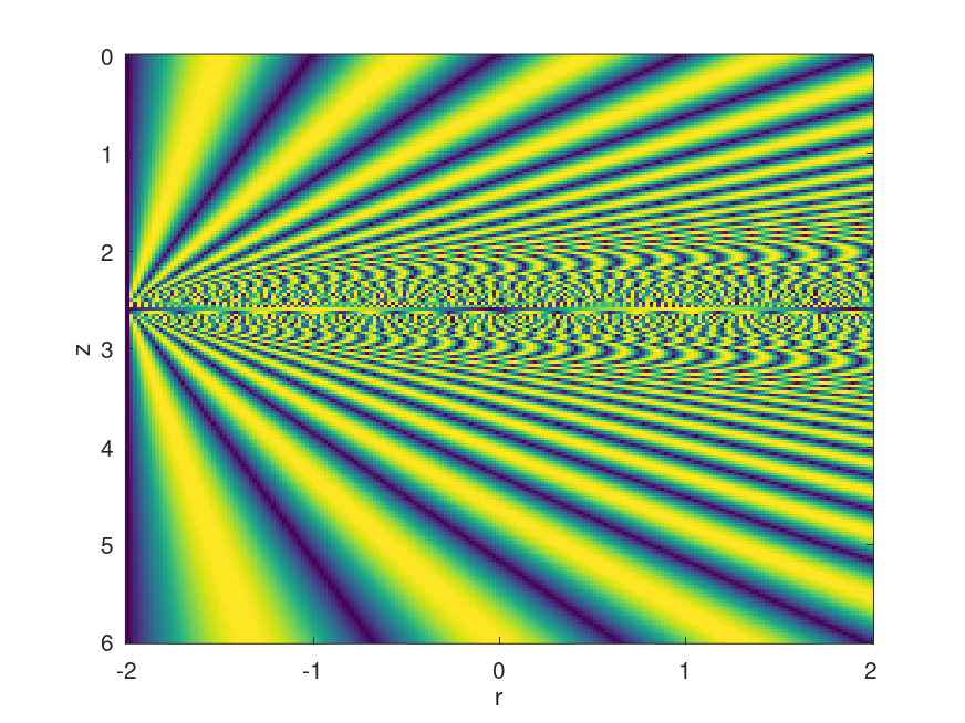
Note: This plot was generated via the waveguide-radial/waveguide_radial_plot.m MATLAB/Octave script in the visualizations/ folder of this repository.

The result is simple: for $\theta >0$, the waves diverge to infinity, and for $\theta <0$, the waves converge at the end of the waveguide ($z=L$), but diverge immediately afterwards to infinity. The only stable configuration that ensures the beam does not diverge is for $\theta =0$. Thus, it makes sense to use a waveguide with a constant radius.