Theoretical analysis of microwave attenuation

This page is to provide an additional theoretical foundation for microwave attenuation, complementing Merits and Limitations of Maser Technology, Literature Review and bringing a more satisfactory answer to this related Codeberg issue. This is essential since the whole premise of space-based solar power is that it is a reliable, all-weather power source that can provide universal 24-hour energy anywhere on Earth. Microwave attenuation is thus a crucial factor in determining the viability of microwave power transmission from space.

Microwave bands

Before we begin, it is useful to introduce the terminology used for denoting different types of microwaves. Microwaves are typically categorized into bands (a band is a range of frequencies) using a letter system, for historical reasons. The typical names for the microwave bands are as follows¹:

Microwave band	Frequency range	Wavelength range
L-band	1 to 2 GHz	15 cm to 30 cm
S-band	2 to 4 GHz	7.5 cm to 15 cm
C-band	4 to 8 GHz	3.75 to 7.5 cm
X-band	8 to 12 GHz	25 mm to 37.5 mm
Ku-band	12 to 18 GHz	16.7 mm to 25 mm
K-band	18 to 26.5 GHz	11.3 mm to 16.7 mm
Ka-band	26.5 to 40 GHz	5 mm to 11.3 mm
Q-band	33 to 50 GHz	6 mm to 9 mm
U-band	40 to 60 GHz	5 mm to 7.5 mm
V-band	50 to 75 GHz	4 mm to 6 mm
W-band	75 to 110 GHz	2.7 mm to 4 mm
F-band	90 to 140 GHz	2.1 mm to 3.3 mm
D-band	110 to 170 GHz	1.8 mm to 2.7 mm

Of the above, everything from the Q-band and above is typically considered part of the millimeter wave range, which has important applications in plasma physics and astronomy, while the L-band contains the so-called 21 cm line, which is the most common astronomical emission line in the Universe, due to the hyperfine transition of atomic hydrogen.

It is commonly understood that S-band and L-band microwaves are minimally attenuated by the atmosphere, even in extremely poor weather conditions, with L-band microwaves. To explain why, however, we must discuss the physical basis of microwave attenuation. We will split this into several sections, because the attenuation of EM waves through the atmosphere is such a complicated topic. In particular, we will cover different mechanisms of atmospheric attenuation in each:

• Gaseous attenuation
• Weather-based attenuation
• Ionosphere-based attenuation
• Other less common forms of attenuation and microwave blockage

Measurements of attenuation

Before we discuss attenuation further, we should note that the typical unit for attenuation is the decibel (dB), which is a logarithmic scale. To convert attenuation in dB to the percentage of power transmitted, we use the following formula:

$$A_{\%}=100\cdot 10^{-A_{\text{dB}}/10}$$

For example, here are the conversions between decibels and linear (percentage) transmission/loss values (rounded to one decimal place, except for the first row):

Attenuation (dB)	Power transmitted (%)	Power loss (%)
0.001	99.98%	0.02%
0.01	99.8%	0.2%
0.1	97.7%	2.3%
0.5	89.1%	10.9%
1	79.4%	20.6%
2	63.1%	36.9%
3	50.1%	49.9%
4	39.8%	60.1%
5	31.6%	68.4%
6	25.1%	74.9%
7	20.0%	80.0%
8	15.8%	84.2%
9	12.6%	87.4%
10	10.0%	90.0%
11	7.9%	92.1%
12	6.3%	93.7%
13	5.0%	95.0%
14	4.0%	96.0%
15	3.2%	96.8%
16	2.5%	97.5%
20	1.0%	99.0%
25	0.3%	99.7%
30	0.1%	99.9%
>30	Essentially 0%	Essentially 100%

Note: An web-based calculator can be found at https://www.desmos.com/calculator/pvewsupdg4.

Since attenuation is distance-dependent, it is also common to give the specific attenuation, which is equal to the attenuation divided by the path length. This is used for calculating free-space path loss: the power loss for microwave transmitters that exists even in vacuum due to diffraction-caused divergence, among other effects. Specific attenuation is also measured in a logarithmic scale, with the typical units of $\mathrm{dB}/\mathrm{km}$, that is, decibels per kilometer (at least for microwave transmission over long distances).

Attenuation due to atmospheric gases

Microwaves are absorbed to varying amounts due to atmospheric gases, due to their absorption spectra. These spectra are generally rotational transitions that can be calculated quantum-mechanically. For instance, water has a major spectral line at 22.3 GHz, ammonia has a spectral line at 24 GHz, and oxygen has a spectral line at 60 GHz (among others).

If water has such strong absorption spectra in the microwave range, a good question is, how do microwaves get through at all? The reason is that there is a major difference between transmitting microwaves into large bodies of liquid water (i.e. trying to send microwaves undersea) and transmitting microwaves through the atmosphere (where we have water droplets and water vapor, but not contiguous liquid water). Liquid water is extremely good at absorbing microwaves, and saltwater is even more so². However, the same is not true for atmospheric water vapor, for reasons we’ll soon see.

This is also an important distinction to be made regarding why sending power down in microwave beams won’t simply “cook” everything in its path, like a microwave oven. The reason is primarily due to the difference in electromagnetic power density. A microwave has a very high electromagnetic power density, given that it concentrates a lot of power (~1 kW) in a relatively small space. However, our design has microwave beams that spread the power over a large area, meaning that the mean power density is much lower.

The overall result is that attenuation due to atmospheric gases is minimal for lower frequencies, particularly in the L-band and S-band. Indeed, models of microwave attenuation (like the ITU-R P.676 model) can be used to simulate the attenuation due to atmospheric gases, and generally predict negligible attenuation.

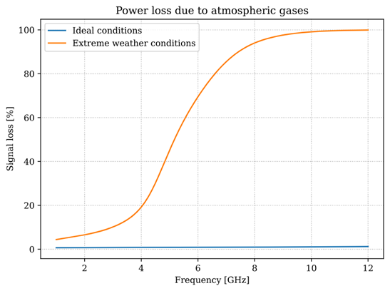
Attenuation due to atmospheric conditions, following the ITU-R P.676 model

Attenuation due to weather

Another significant source of microwave attenuation is due to atmospheric weather. Rain, dust storms, and clouds are the bane of terrestrial solar power, since they block visible light. The commonality between all of these (and several other types of weather) is that they can be modelled as a large collection of particles (we will loosely refer to them as particulates), each of which can scatter electromagnetic waves.

Note that here, we use the word particle to describe a mathematical idealization that represents the real particles in the atmosphere, including rain, hail, dust, ash, suspended water droplets in clouds, snow, and so forth, as well as combinations of them (such as a snow storm, thunderstorm, hurricane, or monsoon). These particles are assumed to be rigid spheres of fixed radius. Of course, this is an approximation, but it turns out to be a pretty good approximation and we don’t need to use the full Navier-Stokes-Maxwell equations to get accurate results.

Attenuation by particles in the atmosphere may be related to the scattering cross-section $\sigma$ with the Beer-Lambert law; the differential form of the Beer-Lambert law is given by the following differential equation:

$$\frac{dI}{dz}=-n\sigma I,I(0)=I_0$$

Where $I$ is intensity of the electromagnetic wave (which is proportional to the square of the electric field), $z$ is the path length (distance through the particulate medium the wave travels), $n$ is the volumetric particle density (in units of particles per unit volume), and $\sigma$ is the cross-section. The solution is given by:

$$I(z)=I_0{e}^{-n\sigma z}$$

In general, there are three mechanisms for the scattering of EM radiation by particulates, characterized by the quantity $\alpha$, where $\alpha =\pi D/\lambda$, $D$ is the particulate diameter and $\lambda$ is the wavelength:

• $\alpha \ll 1$: Rayleigh scattering (particles are much smaller than wavelength)
• $\alpha \approx 1$: Mie scattering (particles are around same size as wavelength)
• $\alpha \gg 1$: Geometric scattering (particles are much larger than wavelength)

Note: In the $\alpha \gg 1$ case, the scattering body is no longer adequately considered as a “particle”; its shape, density, and material composition must be also be considered.

For S-band and L-band microwaves, their wavelengths are so long that $\alpha \gg 1$ is easily satisfied, although Mie scattering has an effect for shorter-wavelength microwaves (particularly millimeter waves). The Rayleigh scattering cross-section is in general a function of angle, particle size, and distance, and we will not show the full cross-section. However, when given as a ratio of the intensity of the scattered wave ($I_s$) compared to the intensity of the incident wave ($I_0$), it tells that:

$$\frac{I_s}{I_0}\sim \frac{r^6}{z^2{\lambda }^4}\sim {\left(\frac{r}{z}\right)}^2{\alpha }^4$$

Where $r$ is the particulate size (for instance, a raindrop), $z$ is once again the path length, $\lambda$ is the wavelength, and $\alpha$ is the same as its previous definition. Once again, for S-band and L-band microwaves, their wavelengths are so long that most particles (including raindrops, snow, and clouds) have absolutely no effect whatsoever³. The same is true for volcanic ash⁴ and dust storms⁵. Hail is a different story, since the largest hailstones can be massive (up to 15 cm!)⁶, although such large hailstones are very uncommon and most hail is small enough to be negligible for L-band microwaves, although they may have still have some effect on S-band microwaves. Starting from the C-band onwards, however, there can be issues.

The conclusion? Atmospheric particles generally have negligible impact on L-band microwaves, and small (but not necessarily negligible) impact on S-band microwaves. However, higher-frequency bands can encounter partial or significant attenuation, and thus are unsuitable for power transmission through the atmosphere.

Other forms of attenuation

While the general consensus is that the atmosphere essentially is transparent to L-band and S-band microwaves, there are specific situations where other forms of attenuation may be present, which we will (briefly) discuss here.

One less-discussed source of attenuation is Tropospheric scattering, a phenomenon where the atmosphere can scatter L-band microwaves due to refraction from water molecules. Tropospheric scattering, however, scatters only a tiny fraction of the incident waves, meaning that it has a minimal effect on power transmission, although extremely sensitive receivers are indeed able to pick up on the lossy signal.

In addition, another form of attenuation, as we’ve briefly mentioned, is free-space path loss - that is, attenuation due to the natural spreading of a collimated microwave beam, which is a fundamental result of the diffraction limit. This is not as much a source of attenuation as a general problem with all focused microwave beams, and we discuss this much further in Combined system efficiency calculations.

Finally, while not exactly “attenuation”, there are so-called reserved frequencies for frequencies used by emergency beacons, distress signals, and passenger aircraft navigation, among others. These frequencies generally cannot be used for space-to-ground links for obvious reasons⁷, meaning that certain frequencies are off-limits despite in theory being non-attenuated.

Mathematical models of attenuation

Attenuation is extremely complicated to model since it is dependent on so many factors, and models of attenuation typically need to be extrapolated from empirical data. The dominant reference to atmospheric attenuation modelling is published by the ITU-R (International Telecommunications Union Radiocommunication Sector) and implemented by software libraries such as ITU-Rpy. Such software can be used to simulate atmospheric attenuation at different locations around the world and in a variety of weather conditions, and provide the most rigorous data on microwave attenuation (other than empirical measurements).

Numerical simulations of attenuation

Using the ITU-Rpy library, we have conducted a large number of simulations of atmospheric attenuation, in a variety of weather conditions: from clear skies and dry air (best) to monsoon weather (worst), and over the entire globe (as attenuation varies geographically due to different climates). The full list of simulations can be found in the notebooks/simulation_data folder of the Elara Labs repository. For instance, the below simulation showcases atmospheric attenuation for 1 GHz microwaves, in normal conditions:

Meanwhile, the following simulation also uses 1 GHz microwaves, but in worst conditions:

It can be seen that there is essentially no difference of atmospheric attenuation despite the different weather conditions for the above two simulations; moreover, even in the worst case, the attenuation is at maximum 0.21 dB, or less than 5% power loss (and in some areas, there is only around 1% power loss). Hence, as expected, L-band microwaves experience minimal (in many cases, essentially negligible) atmospheric attenuation.

We may then contrast this with S-band microwaves, which have a shorter wavelengths compared to L-band microwaves. Specifically, we consider 3.35 GHz microwaves. The below simulation shows the attenuation in normal conditions:

While the following simulation shows the same microwave frequency in worst conditions:

Note: notice that the different atmospheric attenuation simulations have different scaling on the colorbars, which means that initial visual inspection can be misleading, as the same colorscheme is used for all the simulations. The quantitative results (that is, the actual data values) should be used for the correct determination of attenuation, instead of relying only on visual cues.

We immediately notice a substantial difference between the normal and worst-case weather; atmospheric attenuation of S-band microwaves (at least towards the higher-frequency edge of the band) are much more weather-dependent. Moreover, the power loss can be up to 13% in normal conditions and is even greater in the worst conditions. The result is even more prominent with higher-frequency microwaves in the C, X, and Ku bands, with power loss so significant that transmission at acceptable efficiency becomes impossible. Hence, we conclude that L-band and long-wavelength S-band microwaves are most ideal for penetrating the atmosphere and ensuring minimal loss, while short-wavelength S-band microwaves and all the higher bands are to be avoided.

Footnotes

1. See this Wikipedia article, which is based on the conventions of the Radio Society of Great Britain. ↩

2. See Wozniak & Dera (2007), Atmospheric and Oceanographic Sciences Library (ISBN: 978-0-387-30753-4) ↩

3. According to the largest raindrops ever recorded were 8.6 mm across (though possibly larger). This means that they were smaller than a centimeter in size! ↩

4. According to the Volcanic Ashfall Impacts WG from the U.S. Geological Survey ↩

5. See Particle size distribution and particulate matter concentrations during synoptic and convective dust events in West Texas, Aardon-Dryer and Kelley (2022) (DOI: https://doi.org/10.5194/acp-22-9161-2022). ↩

6. According to the NASA Global Precipitation Measurement Mission. ↩

7. A list of the relevant frequencies can be found on the website of the U.S. Code of Federal Regulations. ↩