RF cavity simulation with aperture

An RF cavity is the equivalent of a laser optical cavity; it acts as a resonant chamber for EM waves in the microwave spectrum rather than visible light. It is an essential component of a maser, and can be solved both analytically and numerically, so we detail how to do so below.

The motivation of using RF cavities

The reason why we need to use a RF cavity in a free-electron maser (indeed, among masers in general) is that the cavity is a resonant cavity, meaning that it causes amplification of EM waves. The precise mechanism behind why this amplification occurs is hard to rigorously explain without solving Maxwell’s equations, but the general effect is that an RF cavity is the crucial component necessary to create a maser beam.

In a resonant cavity that is typical for a laser/maser, two mirrors are placed some distance apart, and joined with a tube made of a optically- or microwave-transparent material (depending on the operating wavelength of the laser/maser). This allows EM waves to be reflected between the metal plates, but not reflect off the walls of the tube, which creates a highly-directional and focused beam.¹ This page is not focused on the precise mechanics or engineering of a resonant (optical or RF) cavity; please see Guide to modelling lasers and masers for more information on the topic. Rather, it is focused on describing how to mathematically model and simulate the electromagnetic field inside and outside an RF cavity. Being able to do so will help us design better resonant cavities for high-performance masers.

Note: We will be referring to the RF cavity interchangeably as “RF chamber”, “resonant chamber”, “resonant cavity”, and “resonator”. For our purposes, these are equivalent terminology.

A basic 2D model

Note: Our coordinate conventions are to use $z$ to denote the optical axis (direction of propagation of EM waves), and $r$ to denote the radial distance away from the optical axis, with 2D coordinate points labelled by $(r,z)$. When working in 3D, we use cylindrical coordinates $(r,\varphi ,z)$, where $r,z$ are still defined the same way, and $\varphi$ denotes the azimuthal (angular) coordinate. These are chosen for consistency with our maser coordinates, as well as the typical coordinates used for describing Gaussian beams.

We consider a RF cavity of total width $w$, aperture (hole) width $a_0$, and total length $L$, as shown in the below diagram:

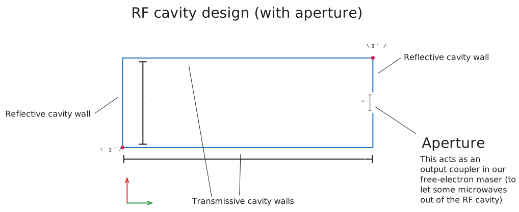
Note: The above diagram is a 2D cross-section. The full 3D cavity (which has a cylindrical shape) is not shown.

Basic analytical solution

To make things simpler, to start, we restrict our analysis to two dimensions only. We also initially assume that there are no longitudinal modes of the electric field (at least, for TE modes). That is to say, we only consider the case where the electric field is transverse (perpendicular) to the optical axis, hence there is only the $E_r$ component of the electric field (at least in our 2D model). The components of the electric field obey the Helmholtz equation $({\nabla }^2+k^2)\mathbf{E}=0$. In our case, this becomes:

$$({\nabla }^2+k^2)E_r=0,E_z=0$$

In our chosen coordinates and in two dimensions, the Helmholtz equation takes the form:

$$\frac{{\partial }^2{E}_r}{\partial z^2}+\frac{{\partial }^2{E}_r}{\partial r^2}+k^2{E}_r=0$$

In two dimensions, it is possible to solve the problem analytically in a fairly straightforward fashion using separation of variables, with the following assumptions:

• The left and right walls of the RF cavity (located at $z=0$ and $z=L$ respectively) are perfect conductors, meaning they reflect all incident EM waves and neither leak nor absorb energy
• The top and bottom walls of the RF cavity (located at $r=-w/2$ and $r=w/2$ respectively) are perfectly transmissive, meaning they allow EM waves to pass through freely
• The aperture is so small as to be negligible in size compared to the width of the RF cavity (that is, $a_0/w\ll 1$), so no energy leaks out the cavity

Note: While it may appear that energy would be needlessly dissipated over the top and bottom walls of the RF cavity, this actually does not happen, since the electromagnetic field quickly becomes zero for $r>R$.

With all of these idealized assumptions, together with the fact that we are ignoring the third dimension, it suffices to say that the results we will obtain will be highly approximate. However, it will prove to be useful before we tackle the much more complex problem of the 3D case, with a non-negligible aperture and non-trivial energy leakage and absorption.

Here, we will not go through the entire process of separation of variables, since it is quite lengthy and is more of an exercise in mathematics than physics or engineering. It suffices to know that after performing the separation of variables procedure, the general solution of the Helmholtz equation in our 2D Cartesian-like coordinates $(r,z)$ is given by²:

$$E_r(r,z)=\sum _{m=1}^{\infty }(A_m{e}^{mr}+B_m{e}^{-mr})[C_m\sin \left(\sqrt{m^2+k^2}z\right)+D_m\cos \left(\sqrt{m^2+k^2}z\right)]$$

We now impose boundary conditions to find a specific solution. We want our solution to apply for all $r$ and all $z\ge 0$, and therefore $A_m$ must be zero, or otherwise the solution blows up at $r\to \infty$. Meanwhile, we impose the requirement that $E_r$ must vanish at the surface of each of the reflective boundary walls (that is, at $z=0$ and $z=L$); this comes from the fact that mirrors are typically made of conductive materials (typically metals), and the tangential components of the electric field at the surface of any perfect conductor is zero. Here, $E_r$ is the tangential component, and therefore $E_r=0$ at both ends of the cavity. To satisfy the $z=0$ boundary condition, $D_m$ must be zero. Now, if we define $K_m=B_m{C}_m$, we have:

$$E_r(r,z)=\sum _{m=1}^{\infty }{K}_m{e}^{-mr}\sin \left(\sqrt{m^2+k^2}z\right)$$

Note: Here, $K_m$ describes the amplitude of the wave as it propagates in space, and depends on the value of $m$. The precise value of $K_m$ can be found through Fourier analysis, but we will not cover this for now.

Meanwhile, to satisfy the $z=L$ boundary condition, we must have $\sin (\sqrt{m^2+k^2}L)=0$. Solving this equation gives us $\sqrt{m^2+k^2}L=n\pi$, or alternatively:

$$k^2=\frac{n^2{\pi }^2}{L^2}-m^2,n=1,2,3,\dots$$

Thus, the modes that the cavity can support are directly related to the integer values of $m$ and $n$, so they are quantized. Now solving for $k$, we obtain:

$$k=\sqrt{\frac{n^2{\pi }^2}{L^2}-m^2},n=1,2,3,\dots$$

We observe that $k$ is only real-valued if $n^2{\pi }^2/L^2\ge m^2$. This means that the minimum value of $m$ is given by the case where $n=1$, that is:

$$m=\frac{\pi }{L}$$

From dimensional analysis we can tell that $m$ has the same units as $k$, and takes the interpretation of a cutoff, prohibiting modes above a certain wavelength³. Indeed, we may define a cutoff wavelength ${\lambda }_c=2\pi /m$, which is given by:

$${\lambda }_c=\frac{2\pi }{(\pi /L)}=2L$$

This is the longest wavelength that the RF cavity permits; it is impossible for any EM wave of a longer wavelength to be present within the cavity. Thus, the RF cavity restricts the possible modes of the electric (and magnetic) fields, allowing us to preferentially select for specific modes. Indeed, if an RF cavity is constructed very carefully to minimize attenuation/losses, then the fundamental mode dominates, and the RF cavity supports EM waves of (almost) purely one wavelength, that being $\lambda ={\lambda }_c$. We can convert this to frequency with $f=c/\lambda$, and thus $f_c=c/{\lambda }_c$. For instance, a $L=10\mathrm{cm}$ RF cavity would therefore have (in our 2D simplification) a fundamental mode with a wavelength of $\lambda =20\mathrm{cm}$, and thus a frequency of around $f=1.5\mathrm{GHz}$⁴.

Additional information: In purely 2D space, there are only TE (transverse electric) modes in the plane of the cavity; a transverse magnetic field must point out of the plane (into the 3rd dimension) and is thus out of our consideration.

Analytical solution with transmissive losses

In our basic model of a maser RF cavity, we assumed that the aperture was negligible in relation to the rest of the cavity. This, of course, is an over-simplification. We will now consider what happens if we do consider the effects of the aperture.

The physical effect of the aperture is that it allows some portion of the electromagnetic field inside the RF cavity to pass outside the cavity. This is a complex process that is not easily modelled analytically. However, we can model it with the following boundary condition (which we may term a transmissive boundary condition):

$$E_r(r,L)=\mathcal{T}{E}_r(r,0)$$

Where $\mathcal{T}$ is the amplitude transmission coefficient, and is a dimensionless number between zero and one that describes what percent of the an electromagnetic wave is allowed to pass outside the RF cavity⁵. Note that we use the curly letter $\mathcal{T}$ rather than the Latin letter $T$ since $T$ is typically used to denote the closely-related power transmission coefficient (the percentage of the power transmitted) defined by:

$$T\equiv \frac{P(z=L)}{P(z=0)}\propto {\mathcal{T}}^2$$

Where $P$ is the power density of the electromagnetic field is proportional to the square of its amplitude. We will not care right now about how exactly one can derive $\mathcal{T}$ or $T$ from first principles, just that it is some known value, and is expressed as the ratio between the electric field’s amplitude at $z=L$ and at $z=0$. That is:

$$\mathcal{T}\equiv \frac{|E_r(r,L)|}{|E_r(0,L)|}$$

Where we require that $\mathcal{T}$ be real-valued, and thus we must take the absolute value, since $E_r$ can be complex-valued. This definition is useless for actually calculating what $\mathcal{T}$ is from first principles, since it requires knowing $E_r$ at the left and right ends of the cavity, which (by definition) we don’t know. However, it can be experimentally-determined by performing actual measurements, or numerically-determined by performing a curve fit on the results of finite-element simulations (more on that later)⁶. We will also later discuss a way to calculate it analytically.

Even if we do not assume a specific form of $\mathcal{T}$, we can recognize some basic qualitative features. In the limit as $a_0\to 0$, then $\mathcal{T}\to 0$, meaning that 0% of the microwaves are transmitted (equivalently, 100% of the microwaves are reflected). This would make for excellent amplification, but would also make it impossible to extract any energy out of the interior of the cavity. Meanwhile, in the limit as $a_0\to w$, meaning that 100% of the microwaves are transmitted (equivalently, none of the microwaves are reflected). This would make the RF cavity equally useless, since all the energy is allowed to pass out of the cavity, and therefore there is no amplification that can happen. But if $\mathcal{T}$ is somewhere in between - for instance, if $\mathcal{T}$ is between 5-10% - it can allow for the RF cavity to still effectively amplify the EM field within, while allowing a reasonable amount of power out of the cavity. We will now solve the problem analytically to show this effect, and solve for the wavelengths (and frequencies) permitted by our waveguide.

Note: Assuming azimuthal symmetry holds, the results of this calculation should be a good approximation (at least in theory) to the modes present in a real, three-dimensional RF cavity.

With our new transmissive boundary condition, let us start at our general solution from before, which was given by:

$$E_r(r,z)=\sum _{m=1}^{\infty }(A_m{e}^{mr}+B_m{e}^{-mr})[C_m\sin \left(\sqrt{m^2+k^2}z\right)+D_m\cos \left(\sqrt{m^2+k^2}z\right)]$$

Once again, we want the solution to be value for all $r$, and therefore $A_m$ must be zero for the solution to not blow up as $r\to \infty$. This gives us:

$$E_r(r,z)=\sum _{m=1}^{\infty }{B}_m{e}^{-mr}[C_m\sin \left(\sqrt{m^2+k^2}z\right)+D_m\cos \left(\sqrt{m^2+k^2}z\right)]$$

This time, we don’t use the perfectly reflective boundary conditions on the left and right wall of the cavity (i.e. setting $E_r\to 0$ at $z=0$ and $z=L$). Instead, we apply our new transmissive boundary condition, giving us (after dropping out common factors):

$$\begin{array}{rl}{C}_m\sin \left(\sqrt{m^2+k^2}L\right)& +D_m\cos \left(\sqrt{m^2+k^2}L\right)\\ & =\cancel{\mathcal{T}{C}_m\sin \left(\sqrt{m^2+k^2}\cdot 0\right)}+\mathcal{T}{D}_m\underset{1}{\underbrace{\cos \left(\sqrt{m^2+k^2}\cdot 0\right)}}\end{array}$$

After simplifying, we obtain:

$$C_m\sin \left(\sqrt{m^2+k^2}L\right)+D_m\cos \left(\sqrt{m^2+k^2}L\right)=\mathcal{T}{D}_m$$

We can remove the (direct) dependency on $C_m$ and $D_m$ by defining a new constant $\rho \equiv \frac{C_m}{D_m}$. Thus, after dividing all sides by $D_m$, we have:

$$\rho \sin \left(\sqrt{m^2+k^2}L\right)+\cos \left(\sqrt{m^2+k^2}L\right)=\mathcal{T}$$

Now solving for $\rho$, we have:

$$\rho =\frac{\mathcal{T}-\cos (\sqrt{m^2+k^2}L)}{\sin (\sqrt{m^2+k^{2}L})}$$

We may rewrite $\rho$ in simpler fashion by defining a new dimensionless quantity $\phi$, such that:

$$\rho (\phi )=\frac{\mathcal{T}-\cos (\phi )}{\sin (\phi )},\phi =\sqrt{m^2+k^2}L$$

What we see is that $\rho$ is negative until $\phi =\pi /2$, after which the sign is switched and we have positive $\rho$. Meanwhile, the first root of $\rho$ is present at $\phi ={\cos }^{-1}$. In addition, at $\phi =n\pi$, the value of $\rho$ asymptotes and therefore $E_r$ is ill-defined. This tells us that it is impossible for $\sqrt{m^2+k^2}L=n\pi$. Finally, if we still assume that the left wall of the cavity (not the right wall!) is sufficiently reflective enough to be near-perfectly-reflective, then it must be the case that at $z=0$ we have $E_r(r,0)=0$, meaning that $D_m=0$ (or otherwise it would be impossible for this to be the case).

All of these conditions together allow us to find the possible modes. By the requirement that $D_m=0$, it necessarily require that $\rho =0$, since $\rho =\frac{C_m}{D_m}$, and thus $\rho D_m=C_m$. This reduces the problem into finding the roots of $\rho (\phi )$ such that for these values of $\phi$, we have $\rho =0$ - equivalently, to find the roots ${\phi }_n^{\ast }$ of $\rho (\phi )$. Now recalling that $\phi \equiv \sqrt{m^2+k^2}L$, we can rearrange to find that:

$$k^2=\frac{({\phi }_n^{\ast }{)}^2}{L^2}-m^2,n=1,2,3,\dots$$

Or equivalently, we have:

$$k=\sqrt{{\left(\frac{{\phi }_n^{\ast }}{L}\right)}^2-m^2},n=1,2,3,\dots$$

Where ${\phi }_n^{\ast }$ (that is the roots of $\rho (\phi )$) can be analytically solved for by solving the transcendental equation $\rho ({\phi }_n^{\ast })=0$, and are given by:

$${\phi }_n^{\ast }=\{\begin{array}{ll}n\pi -{\cos }^{-1}(\mathcal{T}),& n=2,4,6,8,\dots \\ (n-1)\pi +{\cos }^{-1}(\mathcal{T}),& n=1,3,5,7,\dots \end{array}$$

Now again by the requirement that the square root be real, it must be the case that:

$$m^2\le {\left(\frac{{\phi }_n^{\ast }}{L}\right)}^2,{\lambda }_n=\frac{2\pi }{m}=\frac{2\pi L}{{\phi }_n^{\ast }}$$

Therefore, the fundamental wavelength ${\lambda }_c=2\pi /m$ is given by:

$${\lambda }_c=\frac{2\pi L}{{\phi }_1^{\ast }}$$

For $\mathcal{T}\approx 0.1$ (that is, if 10% of the microwaves were allowed to pass out of the cavity) and $L=10\mathrm{cm}$, the first few roots of $\rho (\phi )$ are numerically given by the following table:

Mode	Root (${\phi }_n^{\ast }$)	Fundamental wavelength	Frequency
1st (fundamental)	1.47063	42.7 cm	701.7 MHz
2nd	4.81256	13.1 cm	2.3 GHz
3rd	7.75381	8.1 cm	3.7 GHz

Finally, as a consistency check, let us note that occurs in the limit $\mathcal{T}\to 0$ (where the aperture disappears and both the left and right walls of the cavity become perfectly reflective). In this case, we have:

$$\underset{T\to 0}{\lim }\rho (\phi )=\frac{\sin (\phi )}{\cos (\phi )}=\tan \phi$$

Now setting the requirement that $D_m\to 0$ for both the left and right walls of the cavity (that is, at $z=0$ and $z=L$), as with before, this requires that $\rho =\tan \phi =0$. The roots of $\tan \phi$ are $\phi =n\pi$, and thus we have:

$$k=\sqrt{\frac{({\phi }_n^{\ast }{)}^2}{L^2}-m^2}=\sqrt{\frac{(n\pi {)}^2}{L^2}-m^2},n=1,2,3,\dots$$

Therefore, upon taking the requirement that the square root be real-valued, we have:

$$m=\frac{n\pi }{L}$$

Upon which taking the fundamental ($n=1$) mode gives us:

$${\lambda }_c=\frac{2\pi }{(\pi /L)}=2L$$

This is exactly the result we obtained previously, and shows that our solution is indeed consistent as it reproduces the result of our first derivation in the perfectly reflective, zero-aperture limit.

Analytical 3D model

Now, we will solve the problem in 3D cylindrical coordinates and dispense with the 2D approximation we have used previously. We consider the same cylindrical resonant chamber bounded by two mirrors, but we now consider the case where both have transmissive losses; the power transmission coefficients of the two mirrors are $T_1,T_2$ respectively, meaning that $1-T_1$ and $1-T_2$ (in percent) of power is lost from the two ends of the resonant chamber, respectively. We treat the electric and magnetic fields $\delta \mathbf{E},\delta \mathbf{B}$ of the resonant chamber as a perturbation to the Lorentz force equations (hence the symbol $\delta$ to remind us that it is a perturbation), and we can calculate both from the vector potential $\delta \mathbf{A}$ of the resonant chamber. (Note that we won’t show the calculation of $\delta \varphi$, the (electric) scalar potential, but the same general approach can be used for it).

Why doesn’t a 2D approximation work? The reason is that the Helmholtz equation contains a Laplacian term (that is, ${\nabla }^2$); the Laplacian takes different forms in different coordinate systems, and thus solutions to the Helmholtz equation in different coordinates are distinct. While our 2D solution might suffice as an approximation to a 2D cross-section of the 3D fields, it is still an approximation and is no substitute for a full 3D treatment.

Why use cylindrical coordinates, not rectangular coordinates? The reason is that if we want to form a microwave beam by carefully letting power out of an RF cavity, we must have azimuthal symmetry. Azimuthal symmetry means that cross-sections of the beam are periodic in $\varphi$ (with a period of $2\pi$); otherwise, the “beam” would not be a beam, so to speak, but a propagating plane wave (with cross-sections of squares or rectangles). Cylindrical coordinates naturally incorporates azimuthal symmetry, making it the ideal coordinate system to work in.

Solving for the vector potential

In this case, it is easiest to first solve for the vector potential $\mathbf{A}$ and then obtain the fields from it. Recall that upon a choice of gauge (in our case, the Lorenz gauge is a convenient choice) the vector potential obeys a wave equation. Assuming $e^{i\omega t}$ time dependence, such that $\delta \mathbf{A}(\mathbf{r},t)=\mathbf{A}(\mathbf{r})e^{i\omega t}$ the wave equation reduces to the Helmholtz equation for the vector potential:

$${\nabla }^2\mathbf{A}=-k^2\mathbf{A}$$

Taking advantage of the cylindrical geometry it is convenient to use cylindrical coordinates. Expanding the Helmholtz equation component-wise, we obtain three scalar PDEs, one for each component of $\mathbf{A}$:

$$\begin{array}{r}{\nabla }^2{A}_r=-k^2{A}_r\\ {\nabla }^2{A}_{\varphi }=-k^2{A}_{\varphi }\\ {\nabla }^2{A}_z=-k^2{A}_z\end{array}$$

The solution will now depend on whether the ends of the resonant chamber are curved or flat mirrors. Curved mirrors offer far superior stability, so they are generally used over flat mirrors. However, it is simpler to analyze the case of flat mirrors⁷. We will begin with the general treatment and then proceed to the simpler solution for flat mirrors.

First, note that due to azimuthal symmetry (the solution must repeat every $\Delta \varphi =2\pi$) the angular dependence is simply given by $e^{im\varphi }$ where $m=0,1,2,3,\dots$ is an integer. One thus looks for solutions in the form $A_j(\mathbf{x})=\tilde{A}(r,z)e^{im\varphi }$ where $j\in [r,\varphi ,z]$. Recall the Laplacian in cylindrical coordinates is given by:

$${\nabla }^2=\frac{1}{r}\frac{\partial }{\partial r}\left(r\frac{\partial }{\partial r}\right)+\frac{1}{r^2}\frac{{\partial }^2}{\partial {\varphi }^2}+\frac{{\partial }^2}{\partial z^2}$$

Substituting in our ansatz we obtain:

$${\nabla }^2{A}_j=\frac{1}{r}\frac{\partial }{\partial r}\left(r\frac{\partial }{\partial r}\tilde{A}(r,z)e^{im\varphi }\right)-m^2\frac{\tilde{A}(r,z)e^{im\varphi }}{r^2}+\frac{{\partial }^2}{\partial z^2}[\tilde{A}(r,z)e^{im\varphi }]=-k^2\tilde{A}(r,z)e^{im\varphi }$$

Thus resultingly, we obtain:

$$\frac{1}{r}\frac{\partial }{\partial r}\left(r\frac{\partial \tilde{A}}{\partial r}\right)-\frac{m^2}{r^2}\tilde{A}+\frac{{\partial }^2\tilde{A}}{\partial z^2}=-k^2\tilde{A}$$

Assume $\tilde{A}(r,z)=F(r)G(z)$. We thus have:

$$\begin{array}{c}\frac{1}{r}\frac{\partial }{\partial r}\left(rG{F}^{\prime }(r)\right)+F{G}^{\prime \prime }(z)=\left(\frac{m^2}{r^2}-k^2\right)FG\\ \frac{G}{r}{F}^{\prime }(r)+G{F}^{\prime \prime }+F{G}^{\prime \prime }=\left(\frac{m^2}{r^2}-k^2\right)FG\\ \frac{1}{FG}\left[\frac{G}{r}{F}^{\prime }(r)+G{F}^{\prime \prime }+F{G}^{\prime \prime }\right]=\left(\frac{m^2}{r^2}-k^2\right)\\ \frac{F^{\prime }(r)}{rF(r)}+\frac{F^{\prime \prime }}{F(r)}+\frac{G^{\prime \prime }}{G(z)}=\left(\frac{m^2}{r^2}-k^2\right)\\ \frac{F^{\prime }(r)}{rF(r)}+\frac{F^{\prime \prime }}{F(r)}-\left(\frac{m^2}{r^2}-k^2\right)=-\frac{G^{\prime \prime }}{G(z)}=k^{\prime 2},k^{\prime 2}=\text{const.}\end{array}$$

After some rearrangement, we thus obtain two ODEs:

$$\begin{array}{c}{G}^{\prime \prime }+k^{\prime 2}G=0\\ r^2{F}^{\prime \prime }+r{F}^{\prime }+\left(k^2{r}^2-{\alpha }^2\right)F=0,{\alpha }^2\equiv m^2+k^{\prime 2}\end{array}$$

Where as mentioned prior, $m=0,1,2,3,\dots$ is an integer. The solution for $G$ is evidently a sinusoid, that is:

$$G(z)=B{e}^{i{k}^{\prime }z}$$

Where $B$ is an arbitrary constant; this solution can be checked by substitution. Meanwhile, we identify the ODE for $F$ with the Bessel equation, giving a solution in the form of the Bessel functions of the first kind $J_{\alpha }$:

$$F(r)=C{J}_{\alpha }(kr)$$

Where $C$ is another arbitrary constant. Hence we have:

$$\tilde{A}(r,z)=D{J}_{\alpha }(kr)e^{i{k}^{\prime }z},k^{\prime 2}={\alpha }^2-m^2,D\equiv BC$$

The general solution for $\tilde{A}$ is given by a superposition in the form:

$$\tilde{A}(r,z)=\sum _{\alpha }\sum _{k^{\prime }}{c}_{\alpha }{J}_{\alpha }(kr)e^{i{k}^{\prime }z}$$

Where $c_{\alpha }$ are the coefficients of the series. Note that the full vector potential is given by:

$$\delta \mathbf{A}(r,\varphi ,z,t)={\mathbf{A}}_0\sum _{\alpha =0}^{\infty }\sum _{m=0}^{\infty }\sum _{k^{\prime }}{c}_{\alpha m}{J}_{\alpha }(kr)e^{i{k}^{\prime }z}{e}^{i(m\varphi -\omega t)}$$

Where ${\mathbf{A}}_0$ is the polarization vector of the vector potential, and $c_{\alpha m}$ are (as discussed) the coefficients of the superposition.

Modal decomposition

As we saw above, the general solution for $\mathbf{A}(\mathbf{x},t)$ is a superposition of modes. The modes are parametrized by the integers $\alpha$ and $n$; interestingly, they are not parametrized by wavenumber $k$, as $k$ itself is not quantized since we have imposed open boundary conditions along the sides of the resonator (if the resonator had reflective sides, this would not be true and $k$ would be quantized). We will now turn our attention to the individual modes.

For this, we will start by computing the electric and magnetic fields from the vector potential. Recall that in the absence of an electric potential, the electric and magnetic fields (which we denote by $\delta \mathbf{E}$ and $\delta \mathbf{B}$ respectively) are given by:

$$\delta \mathbf{E}=-\frac{\partial (\delta \mathbf{A})}{\partial t},\delta \mathbf{B}=\nabla \times (\delta \mathbf{A})$$

Substituting our general form of $\delta \mathbf{A}$, we obtain the following series of modes, parametrized by $\alpha$ and $m$:

$$\begin{array}{rl}\delta \mathbf{E}& =-i\omega {\mathbf{A}}_0{J}_{\alpha }(kr)e^{i{k}^{\prime }z}{e}^{i(m\varphi -\omega t)}\\ & ={\mathbf{E}}_0{J}_{\alpha }(kr)e^{i{k}^{\prime }z}{e}^{i(m\varphi -\omega t)}\\ \delta \mathbf{B}& =(i{\mathbf{k}}^{\prime }\times {\mathbf{A}}_0)J_{\alpha }(kr)e^{i{k}^{\prime }z}{e}^{i(m\varphi -\omega t)}\\ & ={\mathbf{B}}_0{J}_{\alpha }(kr)e^{i{k}^{\prime }z}{e}^{i(m\varphi -\omega t)}\end{array}$$

Where we have defined ${\mathbf{E}}_0\equiv -i\omega {\mathbf{A}}_0$ and ${\mathbf{B}}_0\equiv i{\mathbf{k}}^{\prime }\times {\mathbf{A}}_0$, and where ${\mathbf{k}}^{\prime }$ is the wavevector (the same as the $k^{\prime }$ in $e^{i{k}^{\prime }z}$) and is understood to be oriented along $z$. Modes admitted by a resonator are classified as TE (transverse-electric), TM (transverse-magnetic), and TEM (transverse-electromagnetic). These types of modes are characterized by the following table (assuming wave propagation along the $z$ axis):

Mode type	Longitudinal field
TEM	$E_z=B_z=0$
TE	$E_z=0,B_z\ne 0$
TM	$B_z=0,E_z\ne 0$

Note: Here, by “longitudinal field” we mean the component of the fields along the direction of wave propagation (here we choose the $z$ axis, hence the longitudinal components are $E_z$ and $B_z$). The “transverse field” are the components of the fields perpendicular to the direction of wave propagation (i.e. all the components other than $E_z$ and $B_z$).

We will start with the simpler case of a flat mirror to solve for the modes in our cylindrical resonant chamber. Note that the Laguerre-Gaussian modes ${\text{TEM}}_{\ell m}$ are the equivalent for curved mirrors, but they are more complex, so we will leave that discussion for later on. We use a perturbative approach in which we first solve for the case of a lossless resonant chamber, and then add in the effects of losses through the mirrors at the ends of the chamber. This approach requires use of a complex-valued wavevector $k^{\prime }$ and requires that the two mirrors are “good” conductors to begin with (a reasonable assumption in our case).

TEM modes

TEM modes only exist when a non-trivial solution to Laplace’s equation ${\nabla }_T^{2}V=0$ can be found, where ${\nabla }_T^2$ denotes the Laplacian with respect to all the transverse components (i.e. same as the standard Laplacian except without a second derivative w.r.t. $z$). This requires at least 2 conductors to be present (in our case, the mirrors at the ends of the resonator are our conducting surfaces). Interestingly, this means that (hollow) rectangular waveguides and circular waveguides do not have a TEM mode, since they are made of a single conductor; since every point along a conductor is equipotential, the only solution to Laplace’s equation is $V=0$.

Assuming the modes are physically-realizable, one can use a shortcut when evaluating the fields for a TEM mode. This is because the transverse components of the electric field (which we’ll denote as $\delta {\mathbf{E}}_T$) satisfies $\delta {\mathbf{E}}_T=-\nabla (\delta V)$, where $\delta V$ is the electric potential and follows Laplace’s equation ${\nabla }^2(\delta V)=0$. After imposing boundary conditions on $\delta V$ (typically a known voltage on the boundaries or a known gradient of the voltage i.e. electric field on the boundaries) one may solve for $\varphi$, and then take its (negative) gradient to obtain $\delta {\mathbf{E}}_T$. One may then compute the $\mathbf{H}$ field as follows:

$$\delta \mathbf{H}=\frac{1}{Z}\hat{z}\times \delta \mathbf{E},Z=\sqrt{\mu /\epsilon }$$

In linear media, $\mathbf{B}=\mu \mathbf{H}$, hence this can be rearranged to:

$$\delta \mathbf{B}=\hat{z}\sqrt{\epsilon \mu }\times \delta \mathbf{E}$$

In this case, we are working with cylindrical coordinates. However, remember that since here we are interested in the transverse Laplacian, we ignore any derivatives w.r.t. $z$, giving us:

$${\nabla }_T^2=\frac{1}{r}\frac{\partial }{\partial r}\left(r\frac{\partial }{\partial r}\right)+\frac{1}{r^2}\frac{{\partial }^2}{\partial {\varphi }^2}+\cancel{\frac{{\partial }^2}{\partial z^2}}=\frac{1}{r}\frac{\partial }{\partial r}+\frac{{\partial }^2}{\partial r^2}+\frac{1}{r^2}\frac{{\partial }^2}{\partial {\varphi }^2}$$

Hence Laplace’s equation takes the form:

$${\nabla }_T^2(\delta V)=\frac{1}{r}\frac{\partial (\delta V)}{\partial r}+\frac{{\partial }^2(\delta V)}{\partial r^2}+\frac{1}{r^2}\frac{{\partial }^2(\delta V)}{\partial {\varphi }^2}=0$$

We assume a solution in the form $\delta V(r,\varphi )=A(r)B(\varphi )$. Substitution yields:

$$\begin{array}{c}\frac{1}{r}{A}^{\prime }B+A^{\prime \prime }B+\frac{1}{r^2}A{B}^{\prime \prime }=0\\ \frac{1}{AB}\left[\frac{1}{r}{A}^{\prime }B+A^{\prime \prime }B+\frac{1}{r^2}A{B}^{\prime \prime }\right]=0\\ \frac{A^{\prime }}{rA}+\frac{A^{\prime \prime }}{A}+\frac{B^{\prime \prime }}{r^{2}B}=0\\ \frac{r{A}^{\prime }}{A}+\frac{r^2{A}^{\prime \prime }}{A}=-\frac{B^{\prime \prime }}{B}={\ell }^2\end{array}$$

Where ${\ell }^2$ is our separation constant. Upon rearrangement we obtain 2 ODEs:

$$B^{\prime \prime }+{\ell }^{2}B=0,r^2{A}^{\prime \prime }+r{A}^{\prime }-{\ell }^{2}A=0$$

The former is solved with $B(\varphi )=e^{i\ell \varphi }$ as before, for any integer $\ell$. The latter is Euler’s differential equation and solved by:

$$A(r)=c_1{r}^{\ell }\ln r+c_2{r}^{\ell }$$

(Note that here $A(r)$ is just the name of the function and has no relation to the magnetic vector potential). We impose the boundary condition that $V$ must be bounded at all points in the domain (we confine our domain to $r\in [0,R]$ where $R$ is the radius of the resonant cavity). Since $\ln r$ is unbounded as $r\to 0$ we therefore determine that $c_1=0$ and $\ell \ge 0$, leaving us with $A(r)\sim r^{\ell }$. This gives us a series of harmonics $\delta V_{\ell }$ for the harmonics of the potential (where we now write the angular part $e^{i\ell \varphi }$ in real-valued terms):

$$\delta V_{\ell }(r,\varphi )=C{r}^{\ell }\cos (\ell \varphi ),\ell =1,2,3,\dots$$

Where $C$ is an arbitrary constant. The general form is given by a superposition:

$$\delta V(r,\varphi )=\sum _{\ell =1}^{\infty }{C}_{\ell }{r}^{\ell }\cos (\ell \varphi )$$

Where $C_{\ell }$ are the coefficients in the series. The modes of the transverse electric field $\delta {\mathbf{E}}_T=(\delta E_r,\delta E_{\varphi })$ can be straightforwardly found by differentiating the potential, since the electric field is just the negative gradient of the potential (that is, $\mathbf{E}=-\nabla V$). We note that in cylindrical coordinates (with $z$ suppressed) we have:

$$\nabla =\frac{\partial }{\partial r}\hat{r}+\frac{1}{r}\frac{\partial }{\partial \varphi }\hat{\varphi }$$

Hence, the electric field TEM modes are given by:

$$\begin{array}{rl}\delta E_r& =\frac{\partial V_{\ell }}{\partial r}=C\ell r^{\ell -1}\cos (\ell \varphi )\\ \delta E_{\varphi }& =\frac{1}{r}\frac{\partial V_{\ell }}{\partial \varphi }=-C\ell r^{\ell -1}\sin (\ell \varphi ),\ell =1,2,3,\dots \end{array}$$

For the electric field, we let $C=E_0$ be the amplitude of the field. Then, the first few modes are shown in the table below:

Mode	$\delta E_r$	$\delta E_{\varphi }$
$\ell =1$ (fundamental)	$E_0\cos (\ell \varphi )$	$-E_0\sin (\ell \varphi )$
$\ell =2$	$2E_{0}r\cos (\ell \varphi )$	$-2E_{0}r\sin (\ell \varphi )$
$\ell =3$	$3E_0{r}^2\cos (\ell \varphi )$	$-3E_0{r}^2\sin (\ell \varphi )$
$\ell =4$	$4E_0{r}^3\cos (\ell \varphi )$	$-4E_0{r}^3\sin (\ell \varphi )$
$\ell =5$	$5E_0{r}^4\cos (\ell \varphi )$	$-5E_0{r}^4\sin (\ell \varphi )$

The magnetic field components are given by $\delta {\mathbf{B}}_T=\hat{z}\sqrt{\epsilon \mu }\times \delta {\mathbf{E}}_T$. Computing the cross product gives us:

$$\begin{array}{rl}\delta B_r& =-\sqrt{\epsilon \mu }{E}_{\varphi }\\ & =-E_0\sqrt{\epsilon \mu }\ell r^{\ell -1}\cos (\ell \varphi )\\ \delta B_{\varphi }& =\sqrt{\epsilon \mu }{E}_r\\ & =-E_0\sqrt{\epsilon \mu }\ell r^{\ell -1}\sin (\ell \varphi )\end{array}$$

If we define $B_0\equiv \sqrt{E_0^2\epsilon \mu }$ we obtain:

$$\begin{array}{rl}\delta B_r& =-B_0\ell r^{\ell -1}\cos (\ell \varphi )\\ \delta B_{\varphi }& =-B_0\ell r^{\ell -1}\sin (\ell \varphi )\end{array}$$

By definition of being TEM modes, $\delta E_z=\delta B_z=0$. Thus, we have found all 6 components of the electric and magnetic fields.

TE modes

For the TE modes, we have $\delta E_z=0$. This leaves us with the two other components of the electric field to evaluate ($\delta E_r$ and $\delta E_{\varphi }$). Recall our general solution was:

$$\begin{array}{rl}\delta \mathbf{E}& ={\mathbf{E}}_0{J}_{\alpha }(kr)e^{i{k}^{\prime }z}{e}^{i(m\varphi -\omega t)}\\ \delta \mathbf{B}& ={\mathbf{B}}_0{J}_{\alpha }(kr)e^{i{k}^{\prime }z}{e}^{i(m\varphi -\omega t)}\end{array}$$

Where in the case of TE modes in particular, ${\mathbf{E}}_0=(E_{0r},E_{0\varphi },0{)}^T$ and (for reasons we’ll explain shortly) ${\mathbf{B}}_0=(0,0,B_0{)}^T$. For simplicity, we suppress the $e^{-i\omega t}$ time dependence and (as before) take the real part of $e^{im\varphi }$ (which is the physically-measurable part), giving us:

$$\begin{array}{rl}\delta \mathbf{E}& ={\mathbf{E}}_0{J}_{\alpha }(kr)\cos (m\varphi )e^{i{k}^{\prime }z}\\ \delta \mathbf{B}& ={\mathbf{B}}_0{J}_{\alpha }(kr)\cos (m\varphi )e^{i{k}^{\prime }z}\end{array}$$

Assuming an ideal lossless resonant cavity, then the tangential components of the electric field ($\delta E_r$ and $\delta E_{\varphi }$) must vanish at the boundaries ($z=0$ and $z=L$); this is the perfect electric conductor (PEC) boundary condition. For this to be satisfied, we must have $e^{i{k}^{\prime }z}=0$, which lead to the eigenfrequencies defined by $k^{\prime }=k_n^{\prime }\equiv n\pi /L$ for integer $n$, which are purely real-valued. The resonant wavelengths are therefore given by:

$${\lambda }_n^{\prime }=\frac{2\pi }{k_n^{\prime }}=\frac{2L}{n},n=1,2,3,\dots$$

And the resonant frequencies ${\nu }_n^{\prime }$ are given by:

$${\nu }_n^{\prime }=\frac{c}{{\lambda }_n^{\prime }}=\frac{nc}{2L},n=1,2,3,\dots$$

Which is exactly the same as our previous analysis of a lossless cavity! If we substitute in $k^{\prime }=n\pi /L$, the electric field components for the TE modes are thus given by:

$$\begin{array}{rl}\delta E_r& =E_{0r}{J}_{\alpha }(kr)\cos (m\varphi )e^{in\pi z/L}\\ \delta E_{\varphi }& =E_{0\varphi }{J}_{\alpha }(kr)\cos (m\varphi )e^{in\pi z/L}\\ \delta E_z& =0\end{array}$$

Meanwhile, for a perfect conductor, the magnetic field satisfies $\mathbf{B}\cdot \hat{\mathbf{n}}=0$, where $\hat{\mathbf{n}}$ is the normal vector for the conductor’s surface. Hence, the normal component of the magnetic field (in our case, $B_z$) must vanish at the boundaries ($z=0$ and $z=L$). Once again, this leads to the condition that $e^{i{k}^{\prime }z}=0$, resulting in the same eigenfrequencies. Since we are dealing with plane-wave solutions (which are present in the case of flat mirrors), and all plane-wave solutions to Maxwell’s equations must satisfy the orthogonality relation $\mathbf{E}\cdot \mathbf{B}=0$⁸, the remaining components of the magnetic field must be zero. (This is because the electric field is aligned purely along the $r,\varphi$ plane, hence the magnetic field must purely be aligned along $z$ for the orthogonality relation to hold true). Thus the magnetic field components are given by:

$$\begin{array}{rl}\delta B_r& =0\\ \delta B_{\varphi }& =0\\ \delta B_z& =B_0{J}_{\alpha }(kr)\cos (m\varphi )e^{in\pi z/L}\end{array}$$

Now we consider the effect of realistic lossy boundaries. In this case, $k^{\prime }$ becomes complex-valued, and takes the form:

$$k^{\prime }=k_0+i{\alpha }_t,k_0=\frac{n\pi }{L}$$

Where ${\alpha }_t$ is the total attenuation coefficient (not to be confused with the summation index $\alpha$ we used for the Bessel functions in the solution) and $k_0$ is the real part of $k^{\prime }$. Physically-speaking, the imaginary part of $k^{\prime }$ results in an exponential decay $\propto e^{-{\alpha }_{o}z}$ of the waves across the resonator mirrors, as would be expected for lossy boundaries. Moreover, we may write ${\alpha }_t$ as a sum of its contributions from several different effects:

$${\alpha }_t={\alpha }_o+{\alpha }_{dielectric}+{\alpha }_{cond}$$

Where ${\alpha }_o$ describes the intentional loss due to the transmission of energy through the output coupler (aperture), ${\alpha }_{dielectric}$ describes the dielectric loss due to Joule heating (loss of energy through heat), and ${\alpha }_{cond}$ describes the conductive loss due to our imperfect mirrors (which are not perfect conductors)⁹. We can assume ${\alpha }_{dielectric}=0$ as long as the RF cavity is filled with air or vacuum (or a similar material with a relative permittivity of ${\epsilon }_r\approx 1$). The conductive loss and coupling loss, however, should not be ignored. Thus, we have:

$${\alpha }_t={\alpha }_o(T_2)+{\alpha }_{cond}$$

Where the coupling attenuation coefficient ${\alpha }_o$ is a function of the transmission coefficient $T_2$. For a good conductor, the attenuation coefficient is the inverse of its skin depth, and is given by:

$${\alpha }_{cond}\approx \sqrt{\frac{\omega \mu \sigma }{2}}$$

where $\sigma$ is the conductivity of the conductor, $\mu$ is the permeability of the conductor, and $\omega =2\pi f$ is the angular frequency of the wave. Note that $T_1$ (the transmission coefficient of the fully-reflective mirror, which comes only from conductive losses) can also be written implicitly in terms of ${\alpha }_{cond}$ via the Fresnel formula (where we assume normal incidence):

$$T_2=1-{\left|\frac{n_{mirror}-n_{medium}}{n_{mirror}+n_{medium}}\right|}^2=1-{\left|\frac{n_{mirror}-1}{n_{mirror}+1}\right|}^2=\frac{4n_{mirror}}{(n_{mirror}+1{)}^2}$$

Where $n_{mirror}=\sqrt{{\epsilon }_r{\mu }_r}$ is the refractive index of the fully-reflective mirror (which has relative permittivity ${\epsilon }_r$ and relative permeability ${\mu }_r$) and $n_{medium}\approx 1$ is the refractive index of the medium surrounding the cavity (air or vacuum). For metals, the relative permittivity is in general complex-valued, and takes the form:

$${\epsilon }_r=1-\frac{i\sigma }{\omega {\epsilon }_0}=1-\frac{i\sigma }{{\epsilon }_0}\frac{\mu \sigma }{2{\alpha }_{cond}^2}$$

Which can be expressed in terms of our aforementioned expression for ${\alpha }_{cond}$ as:

$$T_2=\frac{4\sqrt{{\epsilon }_r\mu }}{1+{\epsilon }_r\mu +2\sqrt{{\epsilon }_r\mu }},{\epsilon }_r=1-\frac{i\mu {\sigma }^2}{2{\epsilon }_0{\alpha }_{cond}^2}$$

Note that in the limit of a perfect conductor we have ${\epsilon }_r\to 1$ (${\epsilon }_r$ also becomes purely real-valued) and ${\mu }_r\to \infty$, hence $T_2\to 0$ and we have a perfectly-reflective mirror.

The output coupling loss is less easy to describe with a single formula, as it depends on the geometry of the output coupler. Nonetheless, we will aim to obtain an analytical expression for the coupling loss ${\alpha }_o$ in terms of the transmission coefficient $T_2$. To do this, it is useful to note that the electric field magnitude (for constant $r$ and $\varphi$) is given by:

$$\mathbf{E}(z)={\mathbf{E}}_0{e}^{i{k}^{\prime }z}={\mathbf{E}}_0{e}^{i{k}_{0}z}{e}^{-{\alpha }_{o}z}$$

This result does not depend on the choice of $r$ and $\varphi$, since the geometry is axisymmetric. The (electromagnetic) power per unit area is given by:

$$P(z)\propto |\mathbf{E}(z){|}^2\propto |{\mathbf{E}}_0{|}^2{e}^{-2{\alpha }_{o}z}=P_0{e}^{-2{\alpha }_{o}z}$$

Where $P_0\equiv P(0)$ is a constant and is proportional to $|{\mathbf{E}}_0{|}^2$. Notice that the power density decreases with increasing $z$, with the minimum being at $z=L$ which is exactly where the output coupling mirror is. This makes physical sense: power is being transmitted through the output coupling mirror, and therefore is lost from the cavity, with the greatest loss at the same location where power passes out of the cavity. Now, by definition, the transmission coefficient $T_2$ is given by the following ratio:

$$T_2\equiv \frac{P(L)}{P(0)}$$

Hence substituting $P(z)=P_0{e}^{-2{\alpha }_{c}z}$ we obtain:

$$T_2=\frac{P_0{e}^{-2{\alpha }_{o}L}}{P_0}=e^{-2{\alpha }_{o}L}$$

Solving for ${\alpha }_o$, we obtain the following expression for the attenuation coefficient due to output coupling losses:

$$\boxed{{\alpha }_o=-\frac{\ln T_2}{2L},0\le T_2\le 1}$$

Note that an alternative method of calculating the (total) attenuation coefficient, which is more useful in the case of some problems, is to utilize the following formula¹⁰:

$${\alpha }_t=\frac{P_L}{2P_0}$$

Where $P_L$ is the power loss per unit length, $P_0$ is the peak power, and the two are respectively given by:

$$\begin{array}{rl}P(z)& =\int \mathbf{S}\cdot d\mathbf{A}\\ P_L& =-\frac{\partial P}{\partial z}\\ P_0& =P(0)\end{array}$$

Where $\mathbf{S}=\mathrm{Re}\{\mathbf{E}\times {\mathbf{H}}^{\ast }\}=\frac{1}{{\mu }_0}\mathrm{Re}\{\mathbf{E}\times {\mathbf{B}}^{\ast }\}$ is the Poynting vector, ${\mathbf{H}}^{\ast },{\mathbf{B}}^{\ast }$ are the complex conjugates of the $\mathbf{H}$ and $\mathbf{B}$ fields respectively, and the integration is across a cross-section of the cavity. However, this method requires doing integrals and derivatives, so we have elected to use our simpler method.

Finally, we will conclude with an important qualitative observation. While a complex-valued attenuation coefficient ${\alpha }_t$ does change the amplitude of electromagnetic waves in the cavity, it does not change the resonant frequencies (assuming that the attenuation is not too extreme). The presence of a transmissive boundary in the form of an output coupling mirror only leads to a power decay $\propto e^{-{\alpha }_{o}z}$ within the cavity due to the imaginary part of $k^{\prime }$, which is independent of the real part of $k^{\prime }$ that tells us what the resonant frequencies are. Therefore, so long as the perturbative assumption holds, the resonant frequencies ${\nu }_m$ of a cylindrical cavity with plane waves as the standing modes are given by:

$${\nu }_m=\frac{mc}{2L},m=1,2,3,\dots$$

Hence, the resonant frequencies are only dependent on the length $L$ of the resonant cavity (at least theoretically-speaking). Adjusting the length of the resonant cavity will change the resonant frequencies, with a longer resonant cavity leading to a higher-frequency fundamental mode, since ${\nu }_m\propto L^{-1}$.

TM modes

For the TM modes, we have $B_z=0$. Using the same method we have demonstrated above, we obtain the following solutions for the electric and magnetic fields:

$$\begin{array}{rl}\delta E_r& =0\\ \delta E_{\varphi }& =0\\ \delta E_z& =E_{0z}{J}_{\alpha }(kr)\cos (m\varphi )e^{in\pi z/L}\\ \delta B_r& =B_{0r}{J}_{\alpha }(kr)\cos (m\varphi )e^{in\pi z/L}\\ \delta B_{\varphi }& =B_{0\varphi }{J}_{\alpha }(kr)\cos (m\varphi )e^{in\pi z/L}\\ \delta B_z& =0\end{array}$$

The reason that $\delta E_r$ and $\delta E_{\varphi }$ are zero is once again because of the orthogonality condition $\mathbf{E}\cdot \mathbf{B}=0$. Finally, the boundary conditions are the same in the TM case, so we end up with the same resonant frequencies, as well as the same attenuation coefficients.

Laguerre-Gaussian modes

We will now briefly mention the solution for curved mirrors. In the case of ideal curved mirrors, the perturbative fields $\delta \mathbf{E}$ and $\delta \mathbf{B}$ take the form of Laguerre-Gaussian modes. For the electric field:

$$\begin{array}{rl}\delta {\mathbf{E}}_{lp}(r,\varphi ,z)={\mathbf{E}}_0& C_{lp}^{LG}\frac{1}{w(z)}{\left(\frac{r\sqrt{2}}{w(z)}\right)}^{|l|}\exp \left(-\frac{r^2}{w^2(z)}\right)L_p^{|l|}\left(\frac{2r^2}{w^2(z)}\right)\times \\ & \exp \left(-ik\frac{r^2}{2R(z)}\right)\exp (-il\varphi )\exp (i\psi (z))\end{array}$$

Where $l$ and $p$ are integers, $L_p^l(r)$ are the generalized Laguerre polynomials, and $\psi ,w$ are respectively defined as:

$$\begin{array}{rl}w(z)& =w_0\sqrt{1+{\left(\frac{z}{z_R}\right)}^2},z_R\equiv \frac{\pi w_0^2}{\lambda }\\ R(z)& =z\left(1+{\left(\frac{z_R}{z}\right)}^2\right)\\ \psi (z)& ={\tan }^{-1}\left(\frac{z}{z_R}\right)\end{array}$$

Here, $w_0\equiv w(0)$ is the waist radius, and is the width of the main “cone” of radiation within the cavity, and $\lambda$ is the wavelength, which can be calculated from the resonant frequency of the mode using the same formulas as we derived for the plane-wave case. The Laguerre-Gaussian mode solutions are far more complex and not as amendable to perturbative analysis, so we will leave our discussion here.

Exact solution for transmission and reflection coefficients

We have previously assumed a known (empirical) value of the (power) transmission coefficient for the output coupling mirror. It is actually possible to derive an exact solution for the transmission coefficient from first principles. Here, we first define $b\equiv w/2$ for simplicity. Then the power transmitted $P$ in terms of the original power $P_0$ of the beam, assuming a cylindrical RF cavity of diameter $w$ and aperture radius $a_0$ is given by¹¹:

$$P(\theta )=P_0(1-J_0^2(k{a}_0\sin \theta )-J_1^2(k{a}_0\sin \theta ))$$

Where the angle $\theta$ is between the $z$ axis (optical axis) and the radial axis ($r$). The expression given is: and $J_0,J_1$ are the first two Bessel functions. This exact result comes from integrating over the Airy distribution.

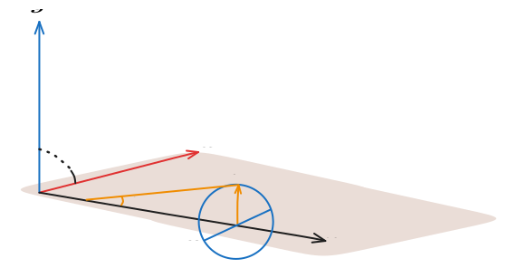
Diagram of the axial conventions used.

From the analytical solution for $P(\theta )$, we can straightforwardly calculate the power transmission coefficient:

$$T=\frac{P(r,L)}{P(r,0)}=1-J_0^2(k{a}_0\sin \theta )-J_1^2(k{a}_0\sin \theta )$$

From this, it is not hard to see that in the case of a very small aperture ($a_0\to 0$) nearly all light is reflected, whereas in the case of a very large aperture ($a_0\to \infty$) nearly all light is transmitted, since:

$$\underset{a_0\to 0}{\lim }T=0,\underset{a_0\to \infty }{\lim }T=1$$

Since the mirror (with the hole in it) has radius $b=w/2$ while the cavity has length $L$, then through simple trigonometry the angle $\theta$ is then $\theta ={\tan }^{-1}(b/L)$. Thus substituting, and noting the well-known identity $\sin [{\tan }^{-1}(x)]=\frac{x}{\sqrt{1+x^2}}$, we get:

$$T=1-J_0^2\left[\frac{k{a}_{0}b}{L\sqrt{1+(b/L{)}^2}}\right]-J_1^2\left[\frac{k{a}_{0}b}{L\sqrt{1+(b/L{)}^2}}\right]$$

Alternatively we can express this in terms of the power reflection coefficient $R$, since $R=1-T$:

$$R=J_0^2\left[\frac{k{a}_{0}b}{L\sqrt{1+(b/L{)}^2}}\right]+J_1^2\left[\frac{k{a}_{0}b}{L\sqrt{1+(b/L{)}^2}}\right]$$

Numerical solution in 2D

To solve the Helmholtz equation numerically, we use the finite element method with the open-source FreeFEM software. This is essential to model physically-realistic cavities that have energy losses. However, in this case, we will not consider such losses in a precise fashion, and find a numerical solution purely based off our simpler model, where we abstract away the precise physics based on a generic transmission coefficient $T$. We interpret $T$ as combining the two sources of power losses:

1. Transmission due to the aperture, which is designed to let out a portion of the microwaves
2. Transmission due to power leakage from the cavity, which is undesirable but nonetheless present in any realistic RF cavity

We will also leave the 3D cylindrical case and other more complex effects for later, and consider the basic 2D Cartesian case only. While this is certainly a very crude model, this numerical simulation is intended to be for familiarization with the concepts of the finite-element method; we will eventually discuss how to perform a numerical simulation that is physically-meaningful and can yield realistic results.

A crash course in the finite element method

Note: This should eventually be ported to the Elara Handbook.

To speak in broad terms, the finite element method approximates a solution to a PDE as a sum of lots of simple piecewise functions called basis functions⁷. If we let ${\psi }_i(\mathbf{x})$ be the $i$-th basis function, and $c_i$ be a constant coefficient to multiply the basis function by, then the solution $E(\mathbf{x})$ can be approximated using the sum of basis functions as:

$$E(\mathbf{x})\approx \sum _i{c}_i{\psi }_i(\mathbf{x})$$

The goal of the finite element is to find the unknown coefficients $c_i$ that best approximate the true solution $E(\mathbf{x})$ of our PDE (the Helmholtz equation). The first step in doing so is to convert the PDE into the variational form (also known as the “weak form”) - essentially, an integral equation that contains the same information as the PDE. We’ll do this in several steps. The first step is to write the PDE in standard form, meaning that we need to move all terms to the left-hand side such that the right-hand side is equal to zero. Luckily, the Helmholtz equation is already in this form:

$${\nabla }^{2}E+k^{2}E=0$$

The next step is to multiply every term of the Helmholtz equation with a test function $\phi$, and integrate the entire left-hand side. A test function is a simple function that has a well-known form, such as a polynomial. This results in:

$${\int }_{\Omega }\phi {\nabla }^{2}E+{\int }_{\Omega }{k}^2\phi E=0$$

Where $\Omega$ denotes the domain in which we’re solving the Helmholtz equation over. Now, the crucial part of the finite element method is that we have to write this integral equation as two terms: one integrated over the domain $\Omega$, and one integrated over the boundary of the domain, which we denote as $\partial \Omega$. To do this, we use integration by parts. Recall that the integration by parts formula in one variable says that:

$${\int }_a^{b}udv=uv{|}_a^b-{\int }_a^{b}vdu$$

The multivariable version of integration by parts takes the form:

$${\int }_{\Omega }udv={\int }_{\partial \Omega }uv-{\int }_{\Omega }vdu$$

Here, we apply integration by parts to our term ${\int }_{\Omega }\phi {\nabla }^{2}E$. Let $u=\phi$ and $dv={\nabla }^{2}E$. Then, we have $du=\nabla \phi$ and $v={\int }_{\Omega }{\nabla }^{2}E=\nabla E$. So using the formula, we get:

$${\int }_{\Omega }\phi {\nabla }^{2}E={\int }_{\partial \Omega }\phi \nabla E-{\int }_{\Omega }\nabla \phi \cdot \nabla E$$

Substituting this result back into the integral equation we got previously, we have:

$${\int }_{\partial \Omega }\phi \nabla E-{\int }_{\Omega }\nabla \phi \cdot \nabla E+{\int }_{\Omega }{k}^2\phi E=0$$

We can combine the two integrals over $\Omega$ and multiply by $-1$ so that we have the simplified result in a specific order, where bilinear (that is, nonlinear) terms come first, and linear terms come after:

$${\int }_{\Omega }\nabla \phi \cdot \nabla E-{\int }_{\Omega }{k}^2\phi E-{\int }_{\partial \Omega }\phi \nabla E=0$$

This is the most general variational form of the Helmholtz equation. The boundary term (the integral over $\partial \Omega$) is the one we’re most interested in, because it depends on our choice of boundary conditions (more on that in the next section). Note that in the finite element world it is common to use the following condensed notation¹²:

$$(\nabla \phi ,\nabla E)-(k^2\phi ,E)-⟨\phi ,\hat{n}\cdot \nabla E⟩=0$$

This comes from the mathematical notation for functional analysis, where the inner product of two functions $f(\mathbf{x}),g(\mathbf{x})$ is denoted $(f,g)$ or $⟨f,g⟩$, and expands to the following integrals:

$$(f,g)={\int }_{\Omega }f(\mathbf{x})g(\mathbf{x}),⟨f,g⟩={\int }_{\partial \Omega }f(\mathbf{x})g(\mathbf{x})\cdot \hat{n}$$

The reason we need to do all this work to get the variational form is that finite element software (like FreeFEM, which we use) can convert this to a matrix equation to solve for $c_i$ using the methods of numerical linear algebra. And since integrals are well-defined even over discontinuous or non-smooth domains (unlike partial derivatives), the variational form used by the finite element method means that you can solve PDEs on very complex geometries, including those with sharp corners, holes, and edges, which are commonly encountered in real-life objects; in such cases, the partial derivatives in the so-called strong form (original differential form) are ill-defined.

Setting up boundary conditions

In our simplified model, we aim to solve for the region $z\in [0,L]$ and $r\in [-R,R]$, where $R>w/2$. To start, we have the transmissive boundary condition from before, where $T$ is a constant:

$$E_r(r,L)=T{E}_r(r,0)$$

In practice, it is easier to set $E_r(r,0)$ to a fixed value and then set $E_r$ based on the transmissive boundary condition. We can set an order-of-magnitude estimate by assuming that the interior electric field is sourced from some spatially and temporally-varying potential source $V(z,t)=V_0{e}^{ikz-i\omega t}$, where $\omega =kc=2\pi c/\lambda$. Therefore, we have:

$$\mathbf{E}=-\nabla V=-\frac{\partial V}{\partial z}=ik{V}_0{e}^{ikz-i\omega t}=V_{0}k{e}^{ikz-i\omega t+i\pi /2}$$

Therefore, the amplitude of the electric field $E_0$ at $z=0$ is given by:

$$E_0=|\mathbf{E}|=V_{0}k=\frac{2\pi V_0}{\lambda }=\frac{2\pi V_{0}f}{c}$$

Making a basic order-of-magnitude approximation for the frequency/wavelength (which can always be refined later), we arrive at a figure for about $42\mathrm{V}/\mathrm{m}$ for $f=1\mathrm{GHz}$ and a $2\mathrm{V}$ power source.

Having placed boundary conditions for the left and right walls, we now need to consider the top and bottom sides of the RF cavity. This is a more complex situation since these regions are open boundaries that allow microwaves to pass unimpeded and radiate away to $r\to \pm \infty$; it is in fact this particular property that allows our RF cavity to be any use at all for use in a maser.

To accurately model outgoing waves that radiate to infinity, we must use the Sommerfeld radiation condition, which, in $d$ dimensions, takes the form:

$$\underset{r\to \infty }{\lim }{r}^{\frac{d-1}{2}}\left(\frac{\partial }{\partial |\mathbf{r}|}-ik\right)E(\mathbf{r})=0$$

Where $r\equiv |\mathbf{r}|$ is the magnitude of the radial vector pointing from the origin of the coordinate system (and is always positive). For instance, the two- and three-dimensional variants of the Sommerfeld radiation condition take the form:

$$\begin{array}{rlr}\underset{r\to \infty }{\lim }\sqrt{r}\left(\frac{\partial }{\partial |\mathbf{r}|}-ik\right)E(\mathbf{r})=0,& & \text{(2D)}\\ \underset{r\to \infty }{\lim }r\left(\frac{\partial }{\partial |\mathbf{r}|}-ik\right)E(\mathbf{r})=0,& & \text{(3D)}\end{array}$$

The requirement for this to be exact, of course, is that the domain is infinitely-large. Of course, we know that simulating infinite domains computationally is impractical. However, we can approximate this boundary condition by surrounding our RF cavity in a large circular region of radius $R$ (shown below), where $R\gg L$ (the circular region is much larger than the RF cavity). Thus, we can say that $R\approx \infty$; it may seem preposterous, but our assumption that $R\gg L$ means that the circular domain can be effectively treated as infinite.

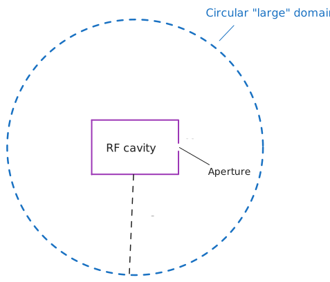
Note: the same general idea can easily be extended into 3D: the only difference is that the circular boundary will need to be changed into a spherical boundary.

We note that since only the top and bottom sides of the RF cavity permit the unimpeded passage of outgoing waves, that is, along the $\pm r$ axes, we must modify the 2D condition to selectively choose the $r$ axis, rather than the general distance $|\mathbf{r}|$. Thus, we have:

$$\underset{r\to \infty }{\lim }\sqrt{r}\left(\frac{\partial }{\partial r}-ik\right)E(r,z)=0$$

If the domain is very large, it is possible to approximate the radiative boundary condition with simpler periodic boundary conditions. See the visualization here for a numerical simulation using periodic boundary conditions (this simulation assumes $T=0$). Indeed, one can approximate the 2D Sommerfeld radiation condition up to first-order with¹³:

$$\frac{\partial E}{\partial r}-ikE=0$$

The solutions to this differential equation over slices of constant $z$ are sinusoids, by inspection; thus this approximation results in plane-waves propagating far away from the sides of the cavity. We will now numerically demonstrate how to compute the electric field. First, recall that our weak form was given by:

$${\int }_{\Omega }\nabla \phi \cdot \nabla E-{\int }_{\Omega }{k}^2\phi E-{\int }_{\partial \Omega }\phi \nabla E=0$$

We now apply our boundary conditions on the third term, which describes an integral performed over the boundaries of the domain the problem is to be solved over. We incorporated the transmissive boundary conditions by setting $E_r(r,0)$ and $E_r(r,L)$ to fixed values with $E_r(r,L)=T{E}_r(r,0)$ and $|E_r(r,0)|=E_0$. These do not affect the boundary term since by nature of being constant values (formally, by being a Dirichlet boundary condition) the gradient of the electric field is zero. However, our open boundaries at $r=-w/2$ and $r=w/2$ do factor in, since they specify a non-vanishing derivative of the electric field at the aforementioned boundaries. Note that since we are considering a 2D domain $\Omega$, the boundary of our 2D domain is a 1D curve, so integrals over $\Omega$ are surface integrals while integrals over $\partial \Omega$ are line integrals. Thus adding the appropriate integral notations, we have:

$$\begin{array}{rl}{\oint }_{\partial \Omega }(\phi \nabla E\cdot \hat{n})d\mathbf{r}& =\underset{r=-w/2}{\oint }\phi \frac{\partial E}{\partial r}d\mathbf{r}+\underset{r=w/2}{\oint }\phi \frac{\partial E}{\partial r}d\mathbf{r}\\ & =\underset{r=-w/2}{\oint }\phi E\left(-\frac{w}{2},z\right)d\mathbf{r}+\underset{r=w/2}{\oint }\phi E\left(\frac{w}{2},z\right)d\mathbf{r}\end{array}$$

Therefore, the weak form of the Helmholtz equation for our chosen boundary conditions (and with the integrals fully written-out) is thus given by:

$${\iint }_{\Omega }(\nabla \phi \cdot \nabla E)dA-{\iint }_{\Omega }{k}^2\phi EdA-\underset{r=-w/2}{\oint }\phi E\left(-\frac{w}{2},z\right)d\mathbf{r}-\underset{r=w/2}{\oint }\phi E\left(\frac{w}{2},z\right)d\mathbf{r}=0$$

Where here, we simulate only the interior field (that is, the field inside the RF cavity itself); we may also simulate both the interior and exterior fields with the circular domain method described previously, but we will omit it for simplicity.

Simulation results

The FreeFEM code for the simulation can be found in freefem/dev/lasers/solve-Efield.edp. The result is shown below:

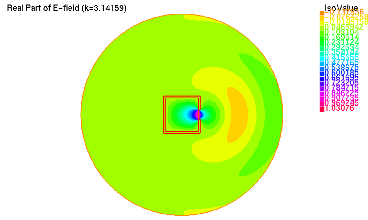
We see some notable features from the simulation. First, the radiation pattern rapidly decays away to infinity and doesn’t stay collimated. This suggests that it would be better to add waveguide to the aperture instead of a bare opening as the output coupler of a maser. Second, as we would expect, the field is zero almost everywhere but the interior of the RF cavity and right in front and around the aperture. Indeed, this is not very different from visible light in a dark room with a small hole in it (see camera obscura).

Note: The code does have some issues right now, including the fact that it is necessary to hard-code a value of the electric field at the aperture (here it is set to $E=E_0=1$) when in theory there should be no physical requirement for this.

The simulation also gives reference values of the electric field strengths for us to compare experimental results against, and thus improve our models. A physically-sound but impractical idea is to put a square plate in front of the maser, with lots of tiny wires crisscrossing the plate. Then, we can measure the voltage across each of the wires at regular intervals to get an approximate idea of the voltage across the entire plate (or we can interpolate numerically). Once we know the voltage $V(x,y)$ we can then figure out the power density (intensity) of the EM waves and compare this against the simulation. The much more practical method is to place a sensitive antenna (or series of antennas) in front of the maser. The antenna(s) can then measure the microwave beam from the maser, much like a radio telescope, allowing us to have an accurate “picture” of how the beam spreads.

Numerical solution in 3D

Note: This section is quite outdated; the numerical solution will use the actual geometry with a PML. See https://pyoomph.readthedocs.io/en/latest/tutorial/spatial/helmholtz.html or equivalent for (Py)MFEM.

Having considered a simplified 2D simulation, we now turn our attention to simulating a realistic cylindrical resonator in 3D. This problem is quite complex and some aspects of it can only be solved numerically, but we will find that analytical methods can get us a long way.

Note: Finite element simulations should be added, with streamline plots and/or vector field plots of both the electric field and magnetic field, as well as the radiation pattern plot (magnitude of the Poynting vector)

To start we can start by once again assuming azimuthal symmetry implicitly, which reduces the 3D problem to a 2D problem, where we use the coordinates $(r,\varphi ,z)$ to denote the transverse (perpendicular to optical axis) and longitudinal (parallel to optical axis) directions, so $E_{\perp }=E_{\perp }(r,z)$ and $E_{\parallel }=E_{\parallel }(r,z)$. The total electric field is then given by $\mathbf{E}=E_{\perp }\hat{r}+E_{\parallel }\hat{z}$.

A typical laser cavity has a 100% reflective mirror on its left end (at $z=0$) and a partially-reflective mirror with reflectivity $\eta <1$ at its right end (it is a bit different for masers but we’ll discuss that later). The electric field satisfies the Helmholtz equation $({\nabla }^2+k^2)\mathbf{E}=0$, which are essentially the time-independent Maxwell equations. When expanded into vector form, this gives us two PDEs to solve:

$$\begin{array}{r}\frac{{\partial }^2{E}_{\perp }}{\partial r^2}+\frac{{\partial }^2{E}_{\perp }}{\partial z^2}+k^2{E}_{\perp }=0\\ \frac{{\partial }^2{E}_{\parallel }}{\partial r^2}+\frac{{\partial }^2{E}_{\parallel }}{\partial z^2}+k^2{E}_{\parallel }=0\end{array}$$

As mentioned, the longitudinal field runs along the optical axis (that is, $E_{\perp }=E_z$), while the transverse field runs perpendicular to it (that is, $E_{\parallel }=E_r$). We assume that the left end (at $z=0$) of the laser cavity has a perfectly-reflective mirror, such that $E_{\perp }=0$ (the tangential component of the electric field is zero, which is true for all perfect conductors). This is equivalent¹ to the following boundary condition:

$$\hat{\mathbf{n}}\times \mathbf{E}=0$$

Where in this case we have $\hat{\mathbf{n}}=\hat{\mathbf{z}}=(0,1{)}^T$. Now, we examine the right side of the laser cavity (at $z=L$). For this side, we have a partially-transparent mirror. This means that the mirror will reflect some light and also transmit some light (we assume no absorption here).

There are several different approaches to this. The first method, and a fairly naive one¹⁴, is to start with the general form of a scattered (plane) wave:

$$u(\mathbf{x})=e^{ik\cdot \mathbf{x}}+r{e}^{-ik\cdot \mathbf{x}}$$

Where $r$ is the reflection coefficient and $R=|r{|}^2$ is the reflectance, or essentially the percentage of light that is reflected. We now consider a generalized mixed boundary condition:

$$c_{1}u(\mathbf{x})+c_2\frac{\partial u}{\partial n}+c_3=0$$

Substituting our solution $u(\mathbf{x})$ in, we have:

$$\begin{array}{c}{c}_{1}u(\mathbf{x})+c_2(ik{e}^{ik\cdot \mathbf{x}}-ikr{e}^{-ik\cdot \mathbf{x}})=-c_3\\ c_1(e^{ik\cdot \mathbf{x}}+r{e}^{-ik\cdot \mathbf{x}})+ik{c}_2(e^{ik\cdot \mathbf{x}}-r{e}^{-ik\cdot \mathbf{x}})=-c_3\\ (c_1+ik{c}_2)e^{ik\cdot \mathbf{x}}+r(c_1-ik{c}_2)e^{-ik\cdot \mathbf{x}}=-c_3\\ r=-\frac{c_3+(c_1-ik{c}_2)e^{ik\cdot \mathbf{x}}}{(c_1+ik{c}_2)e^{-ik\cdot \mathbf{x}}}\end{array}$$

Thus, we have:

$$\begin{array}{rl}R& =|r{|}^2\\ & ={\left|\frac{c_3+(c_1-ik{c}_2)e^{ik\cdot \mathbf{x}}}{(c_1+ik{c}_2)e^{-ik\cdot \mathbf{x}}}\right|}_{(\mathbf{x}=\partial \Omega =L)}^2\\ & ={\left|1+\frac{c_3}{(c_1+ik{c}_2)e^{-ikL}}\right|}^2\end{array}$$

This result is very interesting since it tells us that $c_2<0$ in order for a physically-meaningful reflection coefficient ($R>1$ would violate conservation of energy). Now, the particular values of $c_1,c_2,c_3$ to make this equation true for a certain value of $R$ are actually arbitrary. For simplicity, we can set $c_2=0$ so that we can reduce one of our constants, giving us (for different $c_1$ and $c_3$ than previously):

$$R={\left|1+\frac{c_3}{c_1}{e}^{ikL}\right|}^2$$

Now, let us presume that $c_3=\alpha c_1$, since again the choice of our constants is arbitrary so long as our equation is fulfilled, which also requires that $\alpha <0$. Thus we have:

$$\begin{array}{rl}R& ={\left|1+\frac{\alpha c_1}{c_1}{e}^{ikL}\right|}^2\\ & ={\left|1+\alpha e^{ikL}\right|}^2\\ & =1+{\alpha }^2+2\alpha \cos (kL)\end{array}$$

The solution can be found using the quadratic formula:

$$\begin{array}{c}{\alpha }^2+2\alpha \cos (kL)+(1-R)=0\\ \Rightarrow \alpha =-\cos (kL)-\sqrt{{\cos }^2(kL)-(1-R)}\end{array}$$

Where we take the negative root since we know that $\alpha <0$. This gives us an explicit expression for $\alpha$ in terms of $R,k,L$. Our mixed boundary condition is then:

$$\begin{array}{c}{c}_{1}u(\mathbf{x})+c_2\frac{\partial u}{\partial n}+c_3=0\\ \Rightarrow c_{1}u(\mathbf{x})+\alpha c_1=0\\ \Rightarrow u(L)=-\alpha \end{array}$$

Finally, we obtain our boundary condition:

$$u(L)=\cos (kL)+\sqrt{{\cos }^2(kL)-(1-R)}$$

Where the electric field at the boundary $z=L$ is then given by:

$$\hat{\mathbf{n}}\times \mathbf{E}=u(L)$$

For instance, for a $R=95\%$ reflective mirror and using $\lambda =633\mathrm{nm}$ light, substituting in $k=2\pi /\lambda$ and $L=30\mathrm{cm}$ gives us $|u(L)|=-0.044$. We note that in the special case of $R\to 1$ (that is, all light is reflected), we have:

$$u(L)=\cos (kL)+\sqrt{{\cos }^2(kL)}=\cos (kL)-\cos (kL)=0$$

This is the Dirichlet boundary condition that we would expect for a perfectly-reflective boundary in one dimension. Meanwhile, in the case of $R\to 0$ (that is, all light is transmitted), we have:

$$u(L)=\cos (kL)+\underset{\text{only real for }{\cos }^2(kL)=1}{\underbrace{\sqrt{{\cos }^2(kL)-1}}}=\cos (kL)$$

Which describes outgoing plane waves $u(x)=\cos (kx)=\mathrm{Re}(e^{ikx})$, as we would expect. This is a very crude method and a realistic simulation would most likely use a partially-absorbent boundary condition to model the fact that the mirror at $z=L$ absorbs some light.

Note: in addition to what has been mentioned, realistic laser cavities typically use parabolic/spherical mirrors instead of flat mirrors, so the domain will be curved at either end, making things much more complicated.

Meanwhile, the sides of the laser cavity are usually glass or some other optically-transparent material, making it an open boundary (also called a radiative boundary). This can be modelled by a perfectly-matched layer that allows light to freely pass through. While counterintuitive, this is what maintains the strong directionality of the light along the transmission axis ($+z$) and keeps it as a beam rather than dispersing.

However, a PML requires a bit of work to implement, so it is often easier to just use the first-order approximation of the Sommerfeld radiative boundary condition:

$${\left(\frac{\partial \mathbf{E}}{\partial r}-ik\mathbf{E}=0\right)}_{|r|=R}$$

Putting everything together, we arrive at the following boundary conditions for the electric field inside a laser cavity (although it can be generalized to the outside field as well):

$$\begin{array}{c}{E}_{\perp }(r,0)=0,E_{\perp }(r,L)=\eta E_0\\ \frac{\partial E_{\perp }(z,R)}{\partial r}-ik{E}_{\perp }(z,R)=0,\\ \frac{\partial E_{\perp }(z,-R)}{\partial r}-ik{E}_{\perp }(z,-R)=0,\\ r\in [0,R],z\in [0,L]\end{array}$$

• The aperture has a Sommerfeld-like radiative boundary condition
• The two “mirrors” of the RF cavity (really, they’re just metal plates and don’t have to be polished) have a reflective (homogeneous Dirichlet) boundary condition
• The rest of the RF cavity (including the “tube” connecting the two mirrors) also has a Sommerfeld-like radiative boundary condition; this represents a material transparent to microwaves

In this case, it is easier to use cylindrical coordinates $(r,\Phi ,z)$, where $z$ is the optical axis (direction of propagation) and $(r,\Phi )$ are the radial and polar angles respectively. We again assume our cavity to have length $L$. Our boundary conditions for the Helmholtz equation thus correspond mathematically to:

$$\begin{array}{rlr}& E(r,\Phi ,0)=0,& 0\le r\le R,\\ & E(r,\Phi ,L)=0,& a<r\le R,\\ & \underset{r\to {\infty }^{+}}{\lim }E(r,\Phi ,z)=0,& r>R,\\ & \underset{z\to {\infty }^{+}}{\lim }E(r,\Phi ,z)=0,& 0\le r\le a,\\ & E(r,\Phi ,z)=E(r,\Phi +2\pi ,z),& 0\le \Phi \le 2\pi \end{array}$$

Where our domain is given by $z\in [0,z_{\text{max}}],r\in [0,r_{\text{max}}],\Phi \in [0,2\pi ]$, and we want to pick a suitably large simulation domain (where $z_{\text{max}}\ge 5L$ and $r_{\text{max}}\ge 5R$, roughly) to be able to see both the near-field and the far-field behavior of the beam. Our first two boundary conditions encode the fact that the electromagnetic waves in the cavity must reflect off the two mirrors at each end of the cavity. Meanwhile, our last two boundary conditions encode the fact that the electromagnetic waves must pass freely through the tube connecting the two mirrors, as well as the aperture (output coupler) at the end of the cavity. Our last boundary condition enforces azimuthal symmetry since we expect our solution to be symmetric with respect to $\Phi$. While it may appear that energy would be needlessly dissipated over the sides of the maser, this actually does not happen, since the electromagnetic field quickly becomes zero for $r>R$.

Note: This means that the resultant electric field will be complex-valued; we take only the real part for a physically-meaningful solution.

Maser gain analysis

Lastly, we don’t just want to see what the beam’s wave profile; we also want to know how well the maser amplifies light¹⁵. The corresponding quantity of interest to us in the numerical simulation, which describes this amplification, is called the gain of the maser. The gain compares the output power of the maser to that of an isotropic (point-source) radiator. It is usually measured in decibels (dB), which are a logarithmic unit, and it can be written as:

$$G_{\mathrm{dB}}(\Phi ,\varphi )={\log }_{10}\left(\frac{P_{\text{maser}}(\Phi ,\varphi )}{P_{\text{iso}}(\Phi ,\varphi )}\right)={\log }_{10}\left(\frac{P_{\text{maser}}(\Phi ,\varphi )4\pi |\mathbf{r}{|}^2}{P_{\text{input}}}\right)$$

Where $P_{\text{iso}}=\frac{P_{\text{input}}}{4\pi |\mathbf{r}{|}^2}$ (in cylindrical coordinates we have $|\mathbf{r}|=\sqrt{r^2+z^2}$), $P_{\text{input}}$ is the input power used to drive the maser, the power of the maser is given by $P=|\mathbf{S}|$, and $\mathbf{S}$ is just the Poynting vector. The input power $P_{\text{input}}=(I\Delta V{)}_{\text{input}}$, where $I$ and $\Delta V$ are the driving current and voltage used to power the maser respectively. If we substitute our analytical solution, we find that:

$$P_{\text{maser}}\sim I_0{e}^{-2r^2/a^2},I_0\sim E_0^2$$

Where here, $I_0$ is the maximum intensity of the beam. Thus the gain is approximately:

$$G_{\text{dB}}\sim {\log }_{10}\left(\frac{4\pi I_0|\mathbf{r}{|}^2{e}^{-2r^2/a^2}}{P_{\text{input}}}\right)$$

If we assume that the initial intensity $I_0$ is equal to the input power $P_{\text{input}}$ (that is, we assume that the maser is 100% efficient mechanically-wise), this gives us:

$$G_{\text{dB}}\sim {\log }_{10}(4\pi |\mathbf{r}{|}^2{e}^{-2r^2/a^2})$$

Note that our result is independent of angle and also independent of $z$. However, this is not entirely accurate, as again we are using a simplified solution as opposed to the physically-accurate solution (the Gaussian beam, where $w(z)\ne a$). For a Gaussian beam, the gain becomes:

$$G_{\text{dB}}\sim {\log }_{10}\left(4\pi \frac{(|\mathbf{r}|w_0{)}^2}{w(z{)}^2}{e}^{-2r^2/w(z{)}^2}\right),w_0=a,w(z)\approx \frac{w_{0}z}{L}$$

Where we used the fact that $w(z)\sim z$ for $z\gg L$. This result can be simplified and written explicitly, up to some constants, to:

$$G_{\text{dB}}\sim {\log }_{10}\left(\frac{r^2+z^2}{z^2}{e}^{-2r^2/z^2}\right)\sim {\log }_{10}\left[\left(1+\frac{r^2}{z^2}\right)e^{-2r^2/z^2}\right]$$

It is easy to see that in the limit as $z\to 0$, we have $G_{\text{dB}}\to \infty$. Thus, at its source, a (perfect) Gaussian beam would have effectively infinite gain, which corresponds to infinite amplification of light (once again, here “amplification” means “concentration of energy” not “increasing energy”). Of course, as $z$ increases, the gain of the beam decreases; at some finite distance, $G_{\text{dB}}=0$ (meaning that the Gaussian beam has diverged to the point that it is effectively isotropic and no longer performs useful amplification of light). A minimally-divergent Gaussian beam (whose profile does not change much as $z$ increases) would thus have very high gain; a highly-divergent Gaussian beam would have very low gain. Therefore, decreasing the divergence of a Gaussian beam is absolutely fundamental to improving its amplification and thus its efficiency.

Footnotes

1. This is due to the transverse and longitudinal reflections interfering with each other, leading to the buildup of undesired non-Gaussian modes in the RF cavity. In simplified terms, any off-optical-axis reflections will interfere with the desirable on-axis reflections, causing power to be dispersed and the beam to lose directionality. ↩ ↩²

2. From Wolfram Mathworld’s article article on solving the Helmholtz equation in cartesian coordinates. Owing to our coordinate conventions, we make the substitutions $x\to r,y\to z$. ↩

3. This follows the derivation in Pozar, Microwave Engineering (4th ed.) in Chapter 3.2. ↩

4. For more information, see the Wikipedia article on RF waveguides ↩

5. This was inspired by the boundary conditions described in Freund & Antonssen’s Principles of Free Electron Lasers (4th ed.), ch. 9.1-9.4 as well as the discussion on the transmission coefficient $T_x$ in hole-coupled free-electron lasers from Varro et. al., Free Electron Lasers ,Ch. 3, pg. 68 ↩

6. Directly based off Varro et. al., Free Electron Lasers ,Ch. 3, pg. 68 ↩

7. This is only a basic overview of the finite element method - more details and a much more comprehensive guide to the finite element method can be found on the COMSOL software blog. ↩ ↩²

8. Please see https://farside.ph.utexas.edu/teaching/em/lectures/node48.html for the proof. ↩

9. See Yeap et. al., Propagation in Lossy Rectangular Waveguides (2011) ↩

10. See Cheng (1989), Field and Wave Electromagnetics, Addison Wesley, 0-20152-820-7 ↩

11. See Zen & Ohgaki (2021), J. Opt. Soc. Am. A. The specific equation we reference is eq. 2. ↩

12. This comes from the form shown in the documentation for the pyoomph library. Note that we swap the order of the inner products, but this does not affect the results since the inner product is commutative. ↩

13. Taken from an oomph library example for solving the Helmholtz equation with the finite element method. ↩

14. This is a simplified form of the solution given on Wolfram Mathworld’s article on solving the Helmholtz equation in cylindrical coordinates. In particular, we choose $B_{mn}=F_n=0$ so that the solution does not blow up (become infinite) at $z\to \infty$ and at $z\to 0$. ↩

15. Technically-speaking, a maser (or laser) doesn’t amplify light; at least, not in the sense of producing more (radiant) energy than the energy used to power it. Rather, “amplification” is a rough term that describes the fact that a maser concentrates light so that it is amplified in one particular direction, while reduced in all other directions. ↩