Principles of coherent beam synthesis

Note: We have come to the realization that the technique we have proposed is really just a modification of a phased array, with a few (to our knowledge novel) characteristics:

• We use masers rather than antennas used in traditional phased arrays
• Instead of each individual antenna on the phased array being physically joined together, each maser is on a satellite, and the satellites are spatially separated but fly in formation to form the array
• The system is designed to operate in space

Moreover, it has come to our attention that a very similar technique has been proposed by Bekey (2006) describing a free-flying sparse constellation of satellites to form a phased array.

To be able to realize space-based power beaming, it is necessary to minimize the divergence of laser beams over long distances. Unfortunately, the diffraction limit means that even an idealized single laser beam will diverge at a rate proportional to its wavelength and inversely-proportional to the initial beam radius $w_0$, as given by:

$$\theta =\frac{\lambda }{\pi w_0}$$

Note: see Ideal laser beam divergence for more details and a derivation of this result.

For most lasers, we can make the approximation that $w_0\approx a$, where $a$ is the aperture size of the laser. This means that lasers with small apertures (and thus initially narrow beams) are at a major disadvantage, as their divergence $\theta$ is incredibly-high, even in the ideal case.

To get around this issue is a difficult challenge; after all, we certainly cannot break the laws of physics! However, we can “cheat” by taking inspiration from interferometry and phased arrays. At Project Elara, we have developed a technique — one inspired by existing technologies, but to our knowledge is novel (or at least developed independently) in its specific form — that allows us to functionally focus a beam to narrower than the diffraction limit, while not breaking it per se.

The key to this technique is interference. Like all electromagnetic waves, Gaussian beams can interfere with each other. A superposition of two Gaussian beams from sources (i.e. lasers) located at different positions can constructively and destructively interfere, giving us a combined beam that has peaks and troughs. We will call this combined beam the synthesized beam, and the net effect of the superposition is that the power is concentrated between within a central lobe at the center of the beam, as shown below:

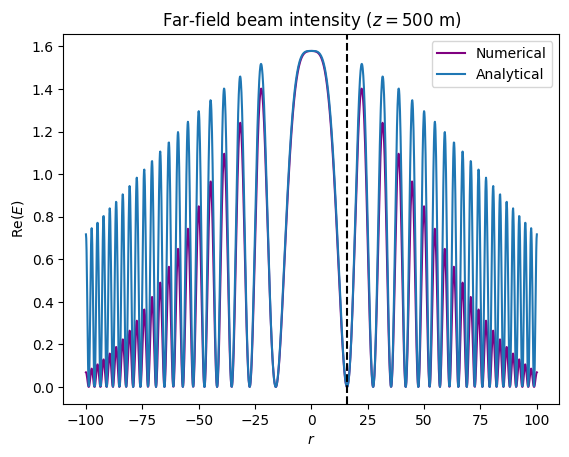
The computed intensity profile of the synthesized beam from two sources spaced 2 meters apart. The calculations are present in notebooks/gaussian-beam-calculations.ipynb

Note: The synthesized beam does not break the diffraction limit because it only alters the beam’s intensity profile, not the divergence of the individual beams themselves, or of the combined beam either.

Mathematical derivation

We will first describe the basic theory, using an introductory derivation — note that this derivation misses some key effects that we will discuss later, hence it is primarily for illustrative purposes. The Gaussian beam is given (in cylindrical coordinates) by:

$$E(r,\varphi ,z)=E_0\frac{w_0}{w(z)}\exp \left(-\frac{r^2}{w(z{)}^2}\right)\exp \left(-i\left(kz+\frac{k{r}^2}{2R(z)}\right)\right)$$

Where we assume that the optical axis (the axis along which the beam propagates) is the $z$ axis, while $r$ is the radial distance from the center of the beam. We consider two Gaussian beams separated by distance $L$ that are aimed at a common spot far away from both lasers. The respective beams then take the forms:

$$\begin{array}{r}{E}_1=E(r_{+}^{\prime },z)\\ E_2=E(r_{-}^{\prime },z)\end{array}$$

Where each beam is pointed at angle ${\theta }_0$, the respective positions of the lasers are at $r=r_{\pm }$, and:

$$r_{\pm }^{\prime }=z\sin {\theta }_0\pm \left(r\mp \frac{L}{2}\right)\cos {\theta }_0$$

However, since the two lasers are aimed at a spot that is very far away, their beams must be near-parallel to the optical axis; otherwise the two beams would cross long before they reach their intended target. This tells us that ${\theta }_0\approx 0$, and thus:

$$r_{\pm }^{\prime }\approx r\mp \frac{L}{2}$$

The synthesized beam then takes the following form:

$$\begin{array}{rl}E(r,z)& =E_1+E_2\\ & =\frac{E_0{w}_0}{w(z)}\left[e^{-i\left(\frac{k{\left(r+\frac{L}{2}\right)}^2}{2R\left(z\right)}+kz\right)}{e}^{-\frac{(r+\frac{L}{2}{)}^2}{w^2\left(z\right)}}+e^{-i\left(\frac{k{\left(r-\frac{L}{2}\right)}^2}{2R\left(z\right)}+kz\right)}{e}^{-\frac{(r-\frac{L}{2}{)}^2}{w^2\left(z\right)}}\right]\end{array}$$

In the far-field limit, where $z\gg L$, then it is possible to use the approximation $r\pm \frac{L}{2}\approx r$. Thus $(\pm \frac{L}{2}+r{)}^2/2R(z)\approx r^2/2R(z)$ and $(\pm \frac{L}{2}+r{)}^2/w(z{)}^2\approx r^2/w(z{)}^2$ so the sum simplifies to:

$$E(r,z)=\frac{2E_0{w}_0}{w(z)}\exp \left(-i\left(\frac{k{r}^2}{2R(z)}+kz\right)\right)e^{-r^2/w^2(z)}$$

Now, to find the physical field from the complex-valued solution, we take the real part of the electric field and discard the imaginary part, giving us:

$$E(r,z)=\frac{2E_0{w}_0}{w(z)}\cos \left(\frac{k{r}^2}{2R(z)}+kz\right)e^{-r^2/w(z{)}^2}$$

We can then find the intensity profile of the beam as follows

$$I=\frac{|E(r,z){|}^2}{2\eta }={\left[\frac{2E_0{w}_0}{w(z)}\cos \left(\frac{k{r}^2}{2R(z)}\right)e^{-r^2/w(z{)}^2}\right]}^2$$

Where $\eta \approx 377\Omega$ is the impedance of free space (or more generally, the impedance of the medium, but we are considering only vacuum for now). We can simplify this by defining:

$$I_0=\frac{2}{\eta }{\left(\frac{E_0{w}_0}{w(z)}\right)}^2$$

Thus our final result is:

$$I(r,z)=I_0{\cos }^2\left(\frac{k{r}^2}{2R(z)}\right)e^{-2r^2/w(z{)}^2}$$

Recall that ${\cos }^2(\theta )=0$ at $\theta =n\pi /2$ where $n$ is an odd integer. Solving for $\frac{\pi }{2}=\frac{k{r}^2}{2R(z)}$ with the far-field approximation $R(z)\approx z$ gives us the positions of the first minima, which are located at the edge of the central lobe. This therefore tells us that the radius (half-width) of the central lobe is given by:

$$r_{min}=\sqrt{\frac{\lambda }{2}z}$$

Note: The diameter $d$ of the central lobe is simply twice this, that is, $d=2r_{min}=\sqrt{2\lambda z}$.

We can verify that this is correct with a simple plot, where we combine the analytical (approximate) solution we derived from evaluating the exact solution for a Gaussian beam numerically:

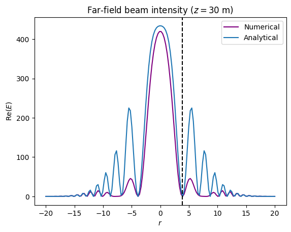
Location of the first minimum is given by the black dashed line. Note how it corresponds perfectly with our result.

We may then calculate the divergence angle $\theta$. Since we have $\tan \theta =r_{min}/z$ and $\tan \theta \approx \sin \theta \approx \theta$ for large $z$ (and thus the small-angle approximation applies) then we have $\theta \approx r_{min}/z=\sqrt{\frac{\lambda }{2}z}/z$. This means that it applies (up to suitable approximations) for any two lasers, even ones with small apertures! Note how this result is remarkably completely independent of the aperture widths of the two individual lasers. We have thus reached our desired result: creating a single synthesized beam that has a divergence angle that does not depend on the apertures of the individual lasers used to create it.

The percentage $r_p$ of power concentrated in the central beam lobe at distance $z=D$ is given by:

$$r_p=\frac{{\int }_{-r_{min}}^{r_{min}}I(r,D)dr}{{\int }_{-\infty }^{\infty }I(r,D)dr}$$

It is possible to analytically solve the two integrals, albeit with much difficulty and with the assistance of a computer algebra system. To start, it is easiest to first define $\alpha =\frac{k}{2R(D)}\approx \frac{k}{2D}$ and $\beta =2/w(D{)}^2$, where $R=R(z)$ and $w=w(z)$ are the same as defined earlier. Therefore, at fixed $z=D$, we have $r_{min}=\sqrt{\frac{\pi D}{k}}\approx \sqrt{\frac{\pi }{2\alpha }}$. Upon substitution and some basic simplifications, we obtain:

$$r_p=\frac{{\int }_{-r_{min}}^{r_{min}}{\cos }^2\left(\alpha r^2\right)e^{-\beta r^2}dr}{{\int }_{-\infty }^{\infty }{\cos }^2\left(\alpha r^2\right)e^{-\beta r^2}dr}$$

The solution to the indefinite integral (ignoring the constant factor of $I_0$) can be expressed in terms of the error function $\mathrm{erf}(x)$ and the imaginary error function $\mathrm{erfi}(z)$ as:

$$\int {\cos }^2\left(\alpha r^2\right)e^{-\beta r^2}dr=\frac{\sqrt{\pi }}{8}\mathrm{Re}\left(\frac{2\text{erf}\left(\sqrt{\beta }r\right)}{\sqrt{\beta }}+\frac{(\beta -2i\alpha )\sqrt{\beta +2i\alpha }\text{erf}\left(r\sqrt{\beta +2i\alpha }\right)+(2\alpha -i\beta )\sqrt{\beta -2i\alpha }\text{erfi}\left(\frac{r(2\alpha +i\beta )}{\sqrt{\beta -2i\alpha }}\right)}{4{\alpha }^2+{\beta }^2}\right)$$

It can also be written in a more compact form using the variables $s$ and $\overline{s}$, where $s=\sqrt{\beta +2i\alpha }$, $\overline{s}=\sqrt{\beta -2i\alpha }$, ${\overline{s}}^2=\beta -2i\alpha$ and $({\overline{s}}^2{)}^{\ast }=2\alpha -i\beta$, as follows:

$$\int {\cos }^2\left(\alpha r^2\right)e^{-\beta r^2}dr=\frac{\sqrt{\pi }}{8}\mathrm{Re}\left(\frac{2\text{erf}\left(\sqrt{\beta }r\right)}{\sqrt{\beta }}+\frac{{\overline{s}}^{2}s\text{erf}\left(sr\right)+({\overline{s}}^2{)}^{\ast }\overline{s}\text{erfi}\left(\frac{r(2\alpha +i\beta )}{\overline{s}}\right)}{4{\alpha }^2+{\beta }^2}\right)$$

Meanwhile, the solution to the definite integral over all space is:

$${\int }_{-\infty }^{\infty }{\cos }^2(\alpha r^2)e^{-\beta r^2}dr=\frac{\sqrt{\pi }}{4}\mathrm{Re}\left(\frac{1}{\sqrt{\beta -2i\alpha }}+\frac{1}{\sqrt{\beta +2i\alpha }}+\frac{2}{\sqrt{\beta }}\right)$$

To explicitly evaluate the real part of $\frac{1}{\sqrt{\beta +2i\alpha }}+\frac{1}{\sqrt{\beta -2i\alpha }}$ we will need to perform a few algebraic manipulations. This can be done by noting that the two fractions are of the general form:

$$\frac{1}{\sqrt{z}}=\frac{1}{\sqrt{x+iy}},x=\beta ,y=\pm 2\alpha$$

Since we know that $z=r{e}^{i\theta }$ then we have $1/\sqrt{z}=1/(\sqrt{r}{e}^{i\theta /2})=\frac{1}{\sqrt{r}}{e}^{-i\theta /2}$. Meanwhile, $r=\sqrt{x^2+y^2}$. The real part of $e^{-i\theta /2}$ is $\cos (-\theta /2)$, which is equal to $\cos (\theta /2)$ since cosine is an even function. Hence, we obtain:

$$\mathrm{Re}\left(\frac{1}{\sqrt{x+iy}}\right)=\frac{1}{\sqrt[4]{x^2+y^2}}\cos \left(\frac{\theta }{2}\right),\theta ={\tan }^{-1}\left(\frac{y}{x}\right)$$

From here, we find that:

$$\mathrm{Re}\left(\frac{1}{\sqrt{x+iy}}+\frac{1}{\sqrt{x-iy}}\right)=\frac{1}{\sqrt[4]{x^2+y^2}}\left[\cos \left(\frac{\theta }{2}\right)+\cos \left(-\frac{\theta }{2}\right)\right]=\frac{2\cos \left(\frac{\theta }{2}\right)}{\sqrt[4]{x^2+y^2}}$$

which is true since ${\tan }^{-1}(x)$ is an odd function and $\cos (x)$ is an even function. Hence:

$$\mathrm{Re}\left(\frac{1}{\sqrt{\beta -2i\alpha }}+\frac{1}{\sqrt{\beta +2i\alpha }}\right)=\frac{2\cos \left(\frac{\theta }{2}\right)}{\sqrt[4]{{\beta }^2+4{\alpha }^2}}$$

And the solution to the integral in closed-form may be expressed as:

$${\int }_{-\infty }^{\infty }{\cos }^2(\alpha r^2)e^{-\beta r^2}dr=\frac{\sqrt{\pi }}{4}\left(\frac{2\cos \left(\frac{\theta }{2}\right)}{\sqrt[4]{{\beta }^2+4{\alpha }^2}}+\frac{2}{\sqrt{\beta }}\right),\theta \equiv {\tan }^{-1}\left(\frac{2\alpha }{\beta }\right)$$

We find that in the limit $z\to \infty$, $r_p\to 1$, meaning that as we go further and further from the source, more and more power is concentrated in the central lobe (although the width of the central lobe does also grow proportional to $\sqrt{z}$). This is very useful because it means that the beam’s power falls off quickly outside the central lobe, meaning that power transmission is much safer, and thus we can use ground receivers that are fairly small (and easy to deploy); even if we are unable to capture the full width of the beam, capturing just the area within the main lobe is sufficient.

Note: Please see this interactive demo showcasing the results we have discussed so far.

Phased-array analysis

Our prior analysis did not explicitly take into account the phase shift between the lasers, and hence we must conduct a more sophisticated analysis to account for it. We can rely on the fact that the system can essentially be described using the same mathematics as a phased array, since — while we use an unusual combination of free-flying array elements (satellites) and use lasers (as opposed to regular antennas) as the RF sources — the above differences should not change the fundamental properties in the far-field¹. The rough equivalent of the divergence angle $\theta$ for a phased array beam is its half-power beamwidth (HPBW), denoted $\Delta \psi$, and also measured in angular units. Assuming a steerable phased array operating at wavelength ${\lambda }_0$, the HPBW can be found from the following implicit equation²:

$$\frac{1}{\sqrt{2}}=\frac{\sin \left(N\left[\frac{\pi d}{{\lambda }_0}\sin \psi -\frac{\Delta \psi }{2}\right]\right)}{N\sin \left(\frac{\pi d}{{\lambda }_0}\sin \psi -\frac{\Delta \psi }{2}\right)}$$

An explicit form for $\Delta \psi$ is approximately given by³:

$$\Delta \psi \approx \frac{0.886{\lambda }_0}{Nd\cos \psi }$$

Where $\psi$ is the beam steering angle, and assuming normal incidence ($\psi =0$) one has $\cos \psi =1$. Note how $\Delta \psi$ is inversely proportional to $d$, the separation between the array elements. Hence, as the array elements are separated by greater and greater distances, the beam becomes far more tightly collimated. For instance, assuming perfect synchronization, a phased array operating at 1 GHz made of $N=10$ elements, separated from each other by a distance of $d=\text{1 km}$, would have a HPBW of $\approx 2.65\times 10^{-5}\text{ rad}$ (or around 5.48 arcseconds), far better than any conventional laser at the same wavelength.

By virtue of being in space our specialized variant of a phased array is far more powerful than a conventional type. This is because, in space, satellites can be placed arbitrarily distant from each other, allowing an array kilometers or even tens of kilometers in size, something that would be impractical to achieve terrestrially. Since the beam divergence $\theta \sim \Delta \psi$ is inversely proportional to the distance $d$ between array elements in a phased array, a very large array can have astoundingly well-collimated beams (with $d$ on the order of tens of kilometers, a divergence of as little as $10^{-6}\text{ rad}$ is possible). Indeed, the technical possibility of Project Elara’s space power beaming relies on this capability.

Engineering considerations

Up to this point, we have only discussed the theory, and not the practical implementation of the design. When considering the actual engineering of the system, we must take into account a few additional considerations.

For instance, conventional phased arrays are typically linear phased arrays (where all array elements are along one line), which have high directivity in-plane, but low-gain out of plane. Instead, we would benefit from a circular phased array (as shown in the diagram below), made by placing several linear arrays branching out from a central hub, like a snowflake’s arms. Due to the azimuthal symmetry, it ensures high directivity both in and out-of-plane.

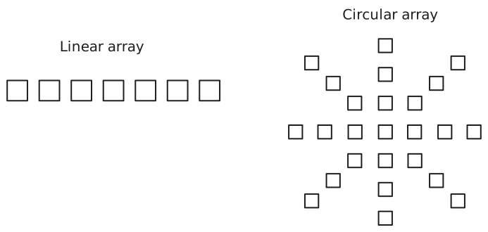
Such a design also has advantages over traditional phased arrays: the fact we use lasers (or more accurately, masers) means that we can achieve a far greater coherence than antennas in traditional phased arrays, and putting masers on satellites allows a very large effective aperture size (and hence a high degree of collimation) without needing to build a power satellite with a massive single aperture kilometers in size. This is especially important because launching anything to space is expensive and highly-complex, hence launching many small satellites is far easier (and more achievable) than launching one giant satellite⁴.

In addition, the fact that our system is just a modified form of phased array means our design is based on decades-old and proven technology. Moreover, it simplifies the process of steering the power beam since phased arrays can steer a beam electronically rather than using mechanical components (e.g. gimbals) that could break down in space.

A major disadvantage, of course, is that the array must be synchronized with near-perfect accuracy to work correctly. In fact, the demands are such that the effects of general relativity may be significant, as the power satellite orbits will precess due to (among other things) GR perihelion precession; this effect, though minuscule, would accumulate over years until (if not corrected) it would alter the satellite orbits enough that they would go out of sync, degrading the phased array.

Appendix: other formulae for similar beams

We can compare the results we arrived for coherent beam-combining with some classic formulae for diffraction-limited beams. For instance, the minimum-diffraction beam that can be made by a perfect lens forms an Airy disk. This result originates in the Fourier optics approach which is rather complicated, so we’ll not discuss it in-depth. However, the end-result is that the radiation pattern of the power density of the electromagnetic field is given (up to some constant factors) by the Airy disk pattern⁵:

$$I(r,z)\sim {\left(\frac{2J_1(a\pi r/\lambda z)}{a\pi r/\lambda z}\right)}^2$$

Where we use $(r,\varphi ,z)$ cylindrical coordinates, $r,z$ are defined in the same way as in the Gaussian beam, $a$ is the aperture width (width as in diameter, not radius), $\lambda$ is the wavelength of the EM waves, and $J_1(\rho )$ is a 1st-order Bessel function of the first kind. You can try an interactive Desmos plot of this radiation pattern; a static plot with $a=0.1,\lambda =1$ is also shown below:

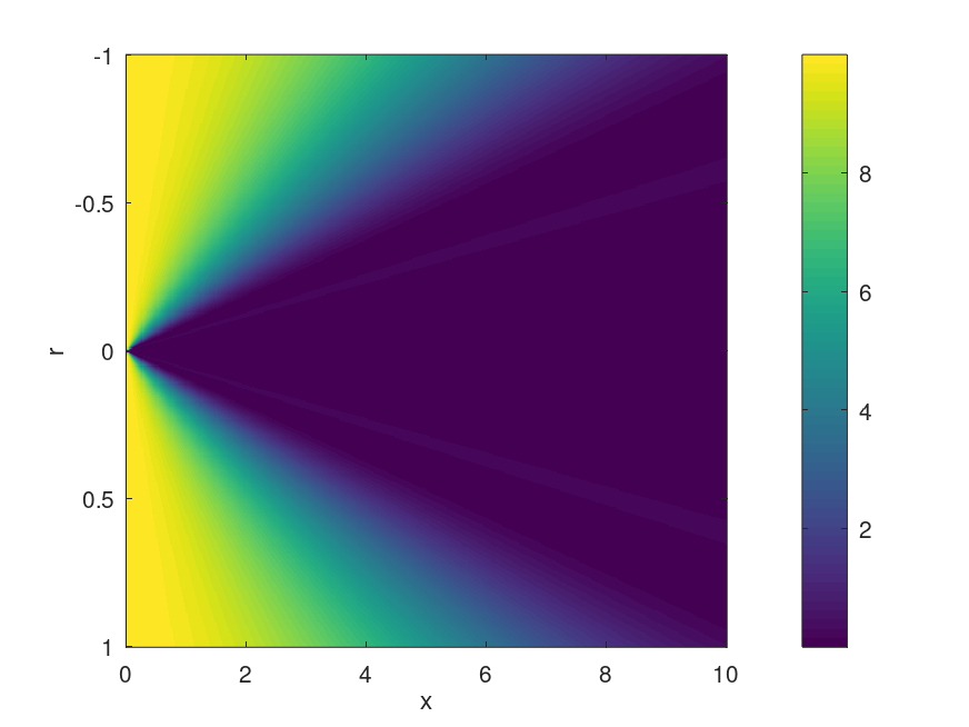
Note: This was generated with the rf-cavity-with-aperture/cavity_with_aperture.m Octave/MATLAB script in the visualizations/ folder of this repository.

The important result is that the wave diverges to infinity and becomes unfocused very quickly after leaving the aperture, which can be seen in the plot, but can also be shown analytically (if we take the limit as $z\to \infty$ we have $I\to 0$ for all $r$). The corresponding formula for its divergence is given by:

$${\theta }_{\text{airy}}\approx 1.22\frac{\lambda }{d}$$

Where $d$ is the diameter of the aperture. Note that for short wavelengths ($\lambda \ll 1$) the formula we derived for the Gaussian beam and that for the Airy disk agree quite closely⁶; this is not surprising, however, given that Airy disks are very similar in principle to Gaussian beams.

This formula is also applicable for astronomical interferometers used for Very-Long Baseline Interferometry, although in some cases the factor of $1.22$ is often dropped to just one, giving the formula⁷:

$${\theta }_{\text{VLBI}}\approx \frac{\lambda }{B}$$

Where $B$ is the baseline distance (the separation between individual telescopes). Unlike our result, neither of these formulas depend on the distance $z$ from the source; however, they are quite similar and illustrate a common property of beam divergence, albeit in different contexts.

Footnotes

1. This is especially true given that while lasers are typically very-high-gain (highly directional) at optical and near-IR wavelengths, this is not true at RF wavelengths, where divergence is so rapid that their beams more resemble the radiation pattern of low-gain (omnidirectional) antennas used in phased arrays rather than optical/IR laser beams. ↩

2. See this article (eq. 12, 13) or its PDF version ↩

3. See Acoleyen et. al., 2009 (eq. 3) ↩

4. See Pozar, Microwave Engineering (4th. ed.) pg. 706. ↩

5. The Airy disk formula comes from this optics website, which additionally goes into more depth about Fourier optics. ↩

6. Interestingly, the results for the Gaussian beam and Airy disk roughly agree up to to around $\lambda =0.5$ (in other words, up to $\text{50 cm}$), which is well into the microwave range. You can check this by plotting the value of $f(\lambda )=|\sqrt{\lambda /2}-1.22\lambda |$ (the factor of $d$ or $L$ is unimportant because $d$ and $L$ are mathematically equal, they just represent different physical things). ↩

7. This formula is taken from the Wikipedia article on angular resolution. It appears that astronomers are satisfied with an order-of-magnitude result for the angular resolution. ↩